ChIP-seq
Peak calling
MACS
MACS is a tool to identify peaks, regions likely bound by targeted protein, in ChIP-seq data. It empirically models the length of the sequenced ChIP fragments, which tends to be shorter than sonication or library construction size estimates, and uses it to improve the spatial resolution of predicted binding sites. Details about the MACS method can also be found here.
The platform provides two versions of the MACS algorithms, 1_3_7 and 1_4_0, whose parameters are explained in the following.
MACS 1_3_7
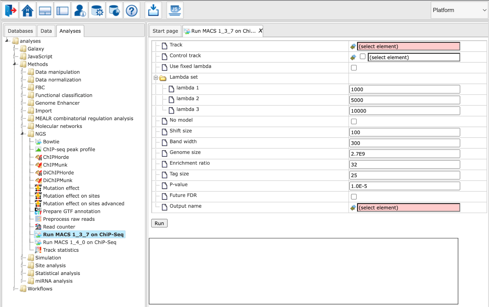
Parameters have the following meanings:
Track: Input track to search for peaks enriched with sequencing tags
Control track: A track that can be used as background (optional)
Use fixed lambda: Use a fixed local lambda for all peak regions
Lambda set: Three scopes of surrounding base pairs to calculate dynamic lambda
lambda 1: close surrounding region
lambda 2: medium width surrounding region
lambda 3: wide surrounding region
No model: Do not build the shifting model. In this mode (no model) a fixed shift size parameter is used.
Shift size: The custom shift size in bp. Used in “no model” mode.
Band width: Expected size of sonicated DNA fragments
Genome size: Effective genome size
Enrichment ratio: Cutoff for the high-confidence enrichment ratio against background
Tag size: Size of sequence tags / read length
P-value: P-value cutoff for peak detection
Future FDR: Adopt the new peak detection method. The default method only considers the peak location in the 1k, 5k, or 10kb regions of the control data. In contrast, the new method also considers the 5k or 10k regions of the test data to calculate the local bias.
Output name: Name of the output track with MACS peaks.
MACS 1_4_0
This is an advanced version of MACS 1.3.7. During model building, the new algorithm selects regions within a certain range of enrichment. By default, permissible enrichment values range from 10 to 30. If MACS fails to build the model, it will resort to “no model”-settings with a shift size=100bps, to shift and extend each tag.
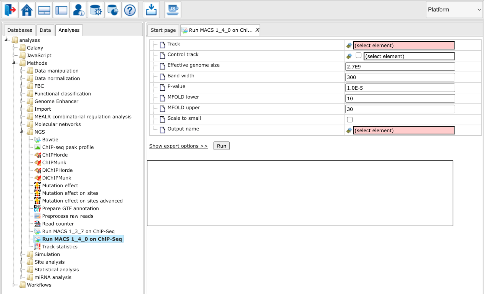
Track: Input track to search for peaks enriched with sequencing tags
Control track: A track that can be used as background (optional)
Genome size: Effective genome size
Tag size (0 = autodetect) (expert): Length of the tag sequences / read length in bp. If set to 0, it will be inferred from average read lengths over several first reads.
Band width: Expected size of sonicated DNA fragments
P-value: P-value cutoff for peak detection
MFOLD lower: Lower bound for high-confidence enrichment ratio used in building the paired-peak model
MFOLD upper: Upper bound for high-confidence enrichment ratio used in building the paired-peak model
Use fixed lambda (expert): Use a fixed local lambda for all peak regions
Small region for dynamic lambda: The close surrounding region (in base pairs) to calculate dynamic lambda. This is used to capture the bias near the peak summit region. Only applied with control data.
Large region for dynamic lambda: The large nearby region (in base pairs) to calculate dynamic lambda. Only applied with control data.
No auto pair process (expert): Whether to turn off the auto pair model process. If marked MACS will exit with an error message if the model building fails. If not marked, it will resort to “no model”-settings
No model (expert): Do not build the shifting model. In this mode (no model) a fixed shift size parameter is used.
Shift size (expert): The custom shift size in bp. Used in “no model” mode.
Keep duplicates (expert): Consideration of replication tags which were assigned to the same genomic location.
Auto: value will be calculated based on binomial distribution using 1e-5 as p-value cutoff
All: Consider all tags
Number: Consider tags at most the specified number of replicated tags
Scale to small: Mark to scale larger dataset down to smaller one
Compute peak profile (expert): Mark to compute a peak profile
Output name: Name of the output track with MACS peaks
SICER
The Galaxy tool SICER fulfills two main purposes:
Delineation of significantly ChIP-enriched regions, which can be used to associate with other genomic landmarks.
Identification of reads on the ChIP-enriched regions, which can be used for profiling and other quantitative analysis.
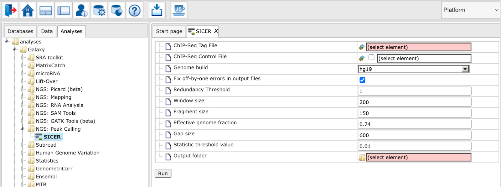
Parameters for SICER should be set as described in the following.
ChIP-Seq Tag File: Input track to search for peaks
ChIP-Seq Control File: A track that can be used as background (optional)
Fix off-by-one errors in output files: SICER creates non-standard output files, this option will fix these coordinates
Redundancy Threshold: The number of copies of identical reads allowed in a library
Window size: Resolution of SICER algorithm. For histone modifications, one can use 200 bp.
Fragment size: For determination of the amount of shift from the beginning of a read to the center of the DNA fragment represented by the read. FRAGMENT_SIZE=150 means the shift is 75.
Effective genome fraction: Effective Genome as fraction of the genome size. It depends on read length.
Gap size: Needs to be multiples of window size. Namely if the window size is 200, the gap size should be 0, 200, 400, 600, …
Statistic threshold value: FDR (with control) or E-value (without control)
Output folder: The output folder contains
“Output summary” table with the fields ChIP_island_read_count, CONTROL_island_read_count, p_value, fold_change and FDR_threshold
A non-redundant version of the input track
A non-redundant version of the control track
A summary file in bedgraph format
A normalized output in Wig format
A track with significant islands
A normalized Wig file with islands
A track with island scores
Output summary: A summary output track with islands
Analyze ChIP-seq peaks
Identify and classify target genes near the peaks
This group of workflows helps to identify genes located near the ChIP-seq peaks or near other genomic intervals. The input can be any track, and the output contains a table of genes overlapping with the fragments of the input track. By default, the gene bound extensions are 10,000 bp 5’ relative to TSS and 10,000 bp 3’ relative to the last exon.
The three workflows in this group have a very similar structure. In the first
step, the input track ( ) is converted into a gene set using the Track to gene set analysis , The resulting Ensembl gene list is then submitted to Functional classification by several ontologies. In parallel, the same Ensembl gene list is subjected to Cluster by shortest path analysis.
The difference between the workflows within this group is in the ontologies applied for functional classification as well as in a database used to find gene/protein clusters, either TRANSPATH® or GeneWays. In the three sections below, three individual workflows are demonstrated using the same input track which can be found [here:]
The results for each of the three workflows can be found in the folder data/Examples/E2F1 binding regions in HeLa cells, ChIP-Seq/Data:
https://platform.genexplain.com/bioumlweb/#de=data/Examples/E2F1%20binding%20regions%20in%20HeLa%20cells%2C%20ChIP-Seq/Data/
Classification by GO categories and metabolic pathways
In this workflow, the functional classification is done using the following ontologies: GO biological processes, GO cellular components, GO molecular function, TF classification, Reactome pathways, and HumanCyc pathways. In parallel, the same Ensembl gene list is subjected to Cluster by shortest path analysis. Gene/protein clusters are calculated based on the GeneWays interaction network.
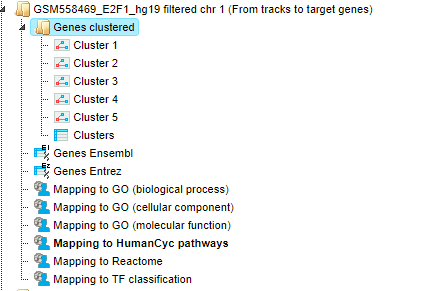
For details, how to launch this workflow, please refer to description of the section classification by GO categories, signaling pathways and diseases. The results folder looks like this:
The input track contains 1889 in vivo binding fragments for E2F1 transcription
factor. These fragments are found to overlap with 2187 Ensembl genes that are
shown in the resulting table Genes Ensembl ( ).
).
Functional classification by the HumanCyc pathways has found 8 metabolic pathways:
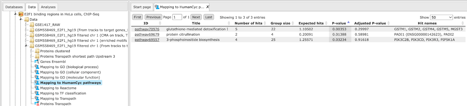
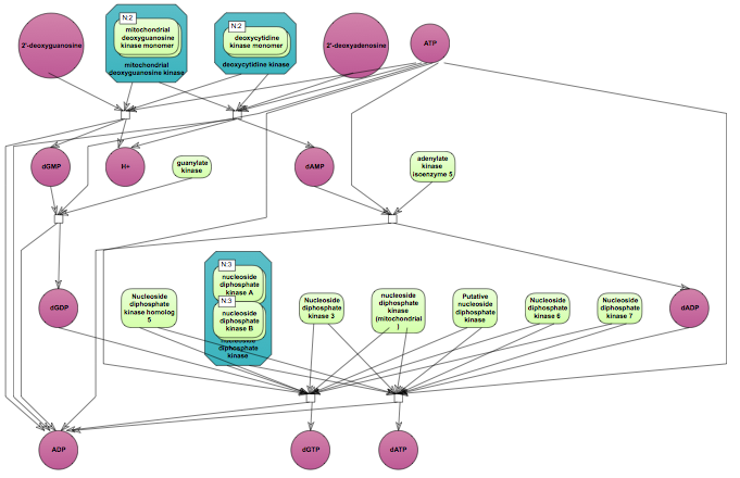
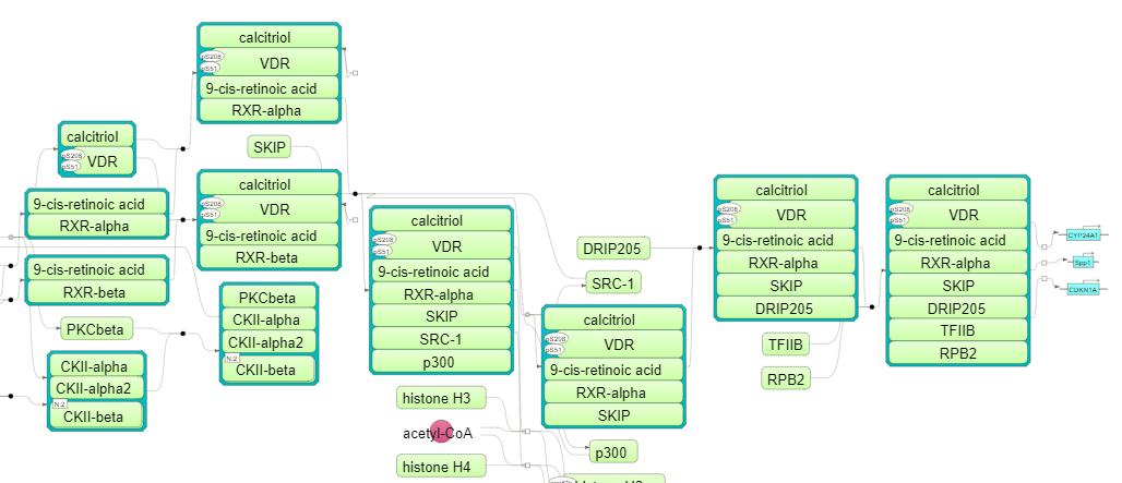
The top pathway visualization diagram can be opened in the work space upon a mouse click to the pathway ID:
The GeneWays clusters are calculated considering upstream direction from the identified with the maximal radius of 2 steps. The following GeneWays clusters are identified:
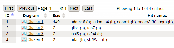
The picture below presents the fragment of the cluster 1.
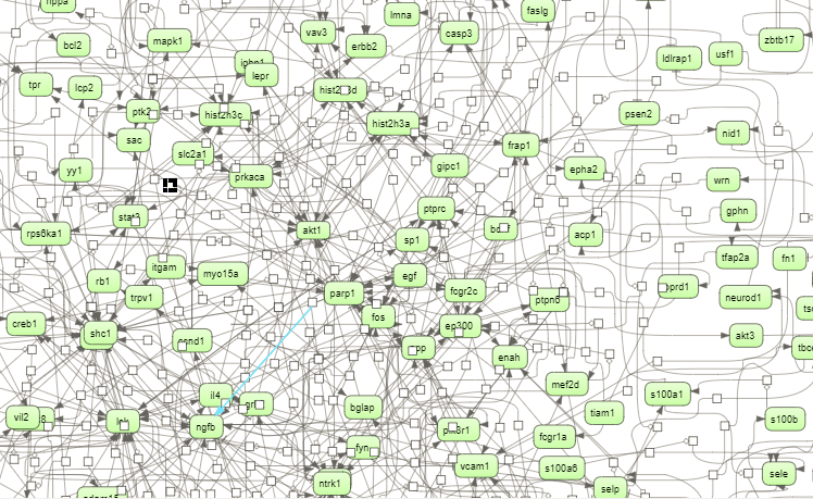
Molecules shown in blue color are coming from the input protein list, and those in green are added by the algorithm when necessary for the connectivity between the elements of the cluster.
Classification by GO categories and signaling pathways
In this workflow, the functional classification is done using the following ontologies: GO biological processes, GO cellular components, GO molecular function, TF classification, Reactome pathways, and TRANSPATH® pathways. In parallel, the same Ensembl gene list is subjected to Cluster by shortest path analysis. Gene/protein clusters are calculated based on the TRANSPATH® signaling network. For the same input as mentioned, the output path for this workflow is:
For details, how to launch this workflow and look into the results, please refer to the description in section Classification by GO categories and metabolic pathways. In our example Functional classification by the TRANSPATH® pathways has found 21 signaling pathways and chains:
The pathway visualization diagrams can be opened in the work space upon a mouse click to the pathway ID. The fragment of the second top pathway, leptin signaling, is shown in force directed layout on the picture below. Important to mention, you can see protein complexes and modified forms on the TRANSPATH® diagrams.
Note This workflow is available together with a valid TRANSPATH® license. Please, feel free to ask for details (info@genexplain.com).
Classification by GO categories, signaling pathway, and diseases
In the first step of this workflow, the input track () is converted into a gene set using the Track to gene set analysis ( ), The resulting Ensembl gene list is then submitted to
Functional classification using the following ontologies: HumanPSD™ GO biological processes, HumanPSD™ GO cellular components, HumanPSD™ GO molecular function, HumanPSD™ disease, TRANSPATH® pathways, TF classification, Reactome pathways, and HumanCyc pathways. In parallel, the same Ensembl gene list is subjected to Cluster by shortest path analysis. Gene/protein clusters are calculated based on the TRANSPATH® network.
), The resulting Ensembl gene list is then submitted to
Functional classification using the following ontologies: HumanPSD™ GO biological processes, HumanPSD™ GO cellular components, HumanPSD™ GO molecular function, HumanPSD™ disease, TRANSPATH® pathways, TF classification, Reactome pathways, and HumanCyc pathways. In parallel, the same Ensembl gene list is subjected to Cluster by shortest path analysis. Gene/protein clusters are calculated based on the TRANSPATH® network.
The input form when opened in the work space is shown below:
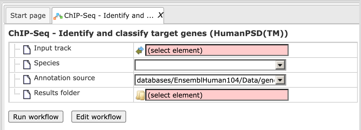
Step 1. Specify input track in BED format in the field Input track.
You can drag & drop it from your project within the tree area. Alternatively, you may click on the pink field select element and a new window will be opened, where you can select the input track.
Here, further steps are demonstrated with the track available here:
Step 2. After input of the track, the species (human, mouse or rat) is adjusted automatically. Verify the species shown in the Species field.
Step 3. Specify the path to store the results and the name of the output folder.
Step 4. Having filled in the input form, launch the analysis with the [Run] button. Wait till the workflow is completed.
Results
The results folder contains several files as shown below. All tables with the resulting classifications as well as the table with clusters and the diagram of the largest cluster are opened by default in the work space.
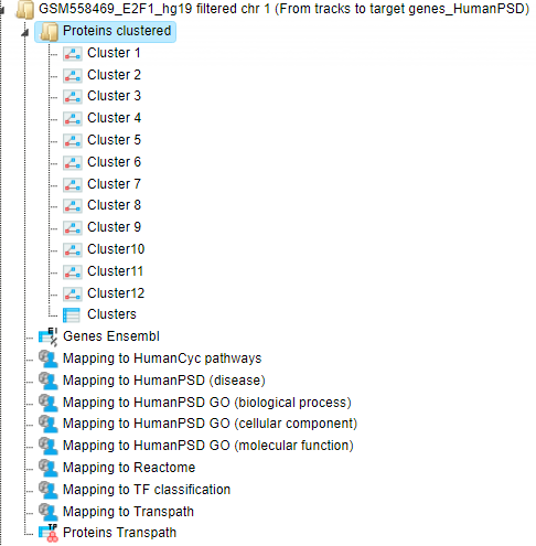
The table Genes Ensembl () contains those genes that are identified as located in the regions around the input peaks or fragments. By default this workflow considers the following
regions around Ensembl genes: 10000 bp in 5’ direction from TSS and 10000 bp in
3’ direction from the last exon. The positions of each fragment on the input
track are compared with positions of the extended gene regions. Genes
overlapping with at least one input fragment are considered as resulting target
genes. For the input track in this example, 2187 Ensembl genes are identified.
The resulting table Genes Ensembl is shown below, sorted by the column
Count.
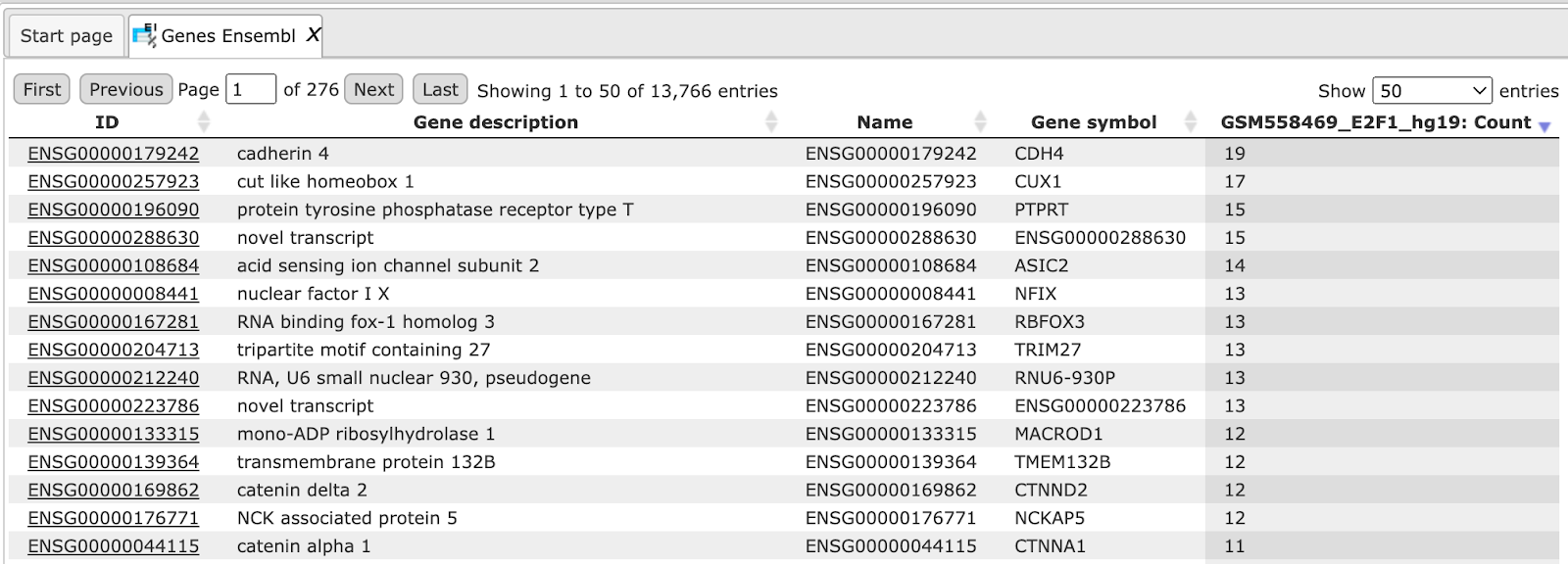
Each row in this table contains information about one identified gene including Ensembl gene ID, chromosome, exact genomic positions and strand (1 or -1), gene symbol, and description. The column Count shows how many fragments on the input track are overlapping with each gene.
These genes are then converted into TRANSPATH® proteins, the output table Proteins Transpath is, shown below:
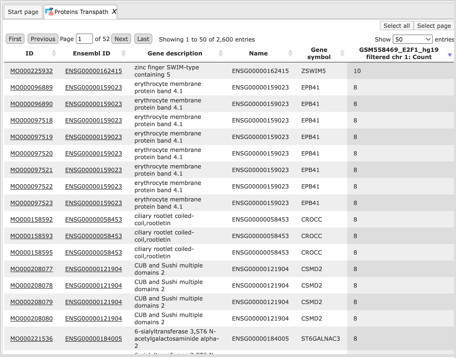
The structure of this table is very similar to that of Genes Ensembl, the critical difference is the column ID, which represents TRANSPATH® molecule IDs; Ensembl gene IDs are given in the second column. Here 1594 Ensembl genes are converted into 1065 TRANSPATH® proteins.
Resulting TRANSPATH® proteins are clustered to get functional connections between the gene products. By default, the workflow considers upstream direction from the input TRANSPATH® proteins with a radius of 3. Resulting clusters are present in the folder Proteins clustered, shown below.
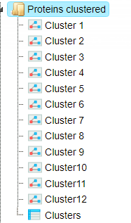
The table Clusters ( ) contains a list of all identified clusters, here 12. Each row shows details
for one cluster. The clusters are sorted by their size with the largest cluster on top. The column Hit names contains names of TRANSPATH® proteins in each cluster.
) contains a list of all identified clusters, here 12. Each row shows details
for one cluster. The clusters are sorted by their size with the largest cluster on top. The column Hit names contains names of TRANSPATH® proteins in each cluster.
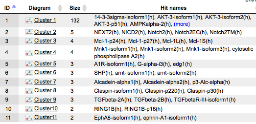
A visualization of the largest cluster, Cluster 1, is opened automatically when the workflow is completed. The visualization of Cluster 1 in orthogonal layout is shown below:
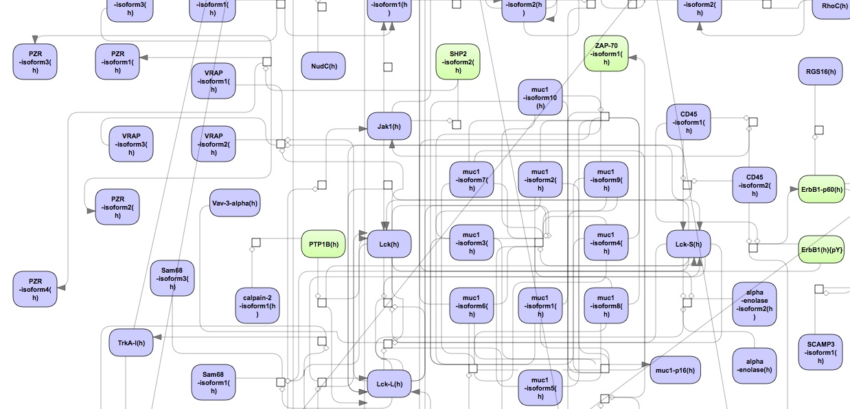
Molecules shown in blue color are coming from the input protein list, and those in green are added by the algorithm when necessary for the connectivity between the elements of the cluster.
In parallel with clustering, the table Genes Ensembl undergoes to Functional
classification. The results are shown in eight tables with the icon ( ). Each table corresponds to a separate ontological category used for the classification in this workflow.
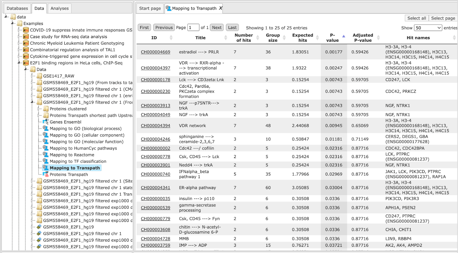
The resulting table, e.g. Mapping to HumanPSD GO (disease), looks like this:
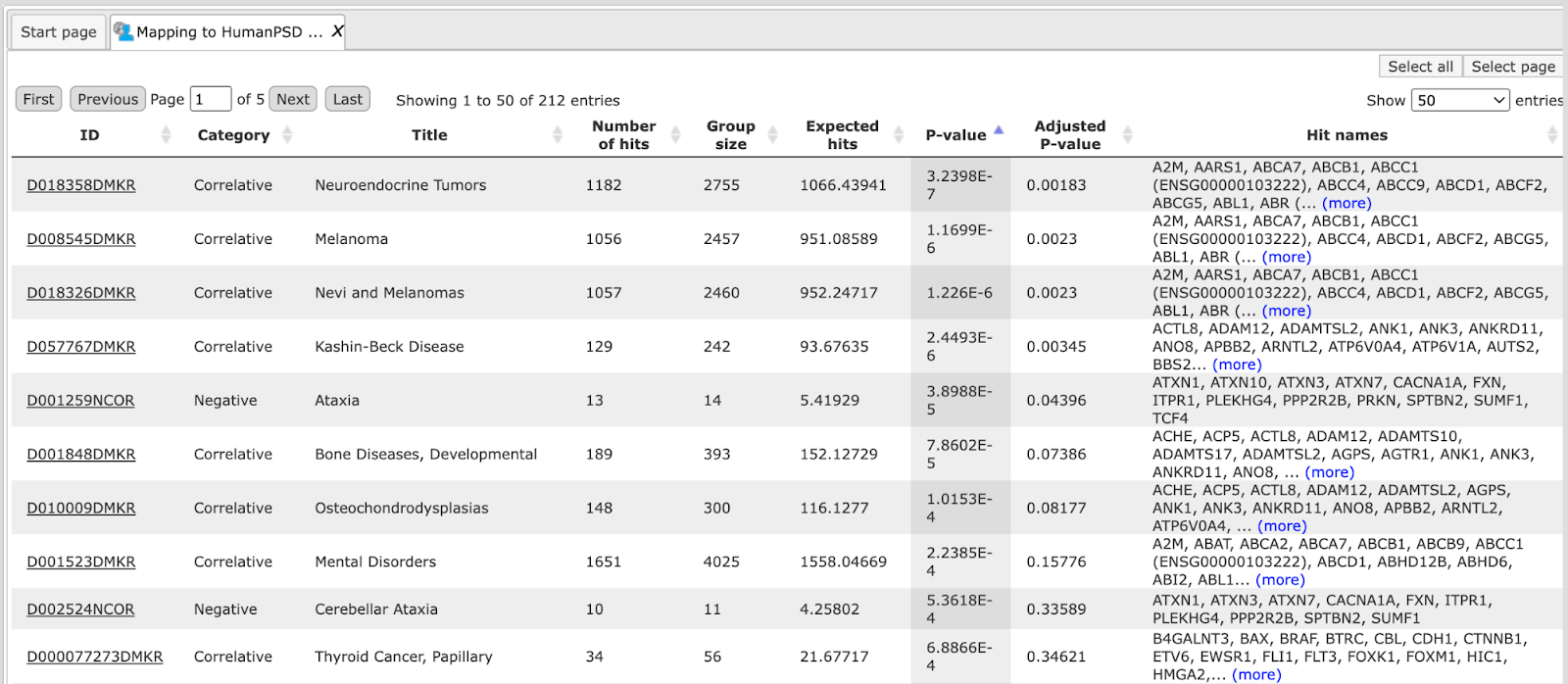
Each row corresponds to one ontological category, which in this case is one of the diseases as they are annotated in the HumanPSD™ database. Commonly accepted disease identifiers are shown in the ID column. The disease names are shown in the column Title. The column Group size represents the number of genes linked to this disease in HumanPSD™, and the column Category demonstrates the functional type of the link between genes and disease; it can be causal, correlative or negative. For each row several parameters are calculated, the expected number of hits (Expected hits), the actual number of hits (Number of hits), P-value, as well as Hit names. IDs are hyperlinked to an external web page of CTD, the Comparative Toxicogenomics Database. With a click on each ID, a new tab will be opened displaying additional information about the disease.
Note This workflow is available together with a valid HumanPSD™ license. Please, feel free to ask for details (info@genexplain.com).
Site search with TRANSFAC®
Version 2.0 (Adjusted p-values, site search on track)
Single interval list
This workflow “Identify enriched motifs in tracks (TRANSFAC®)” is designed to
map putative enriched TFBSs on peaks calculated from your ChIP-seq data (Yes
set) as compared to a random background set (No set). Importantly, the No set is
created automatically and contains by default 1000 intervals. In the first part
of the workflow, the enriched motifs are identified by our proprietary MEALR
approach (analyses/Methods/Site analysis/MEALR (tracks), icon ( ).
).
Enriched motifs serve as a basis to construct a specific profile. At the next
step this newly generated profile is run on the same list of input peaks
applying the method analyses/Methods/Site analysis/Search for enriched TFBSs
(tracks), icon (
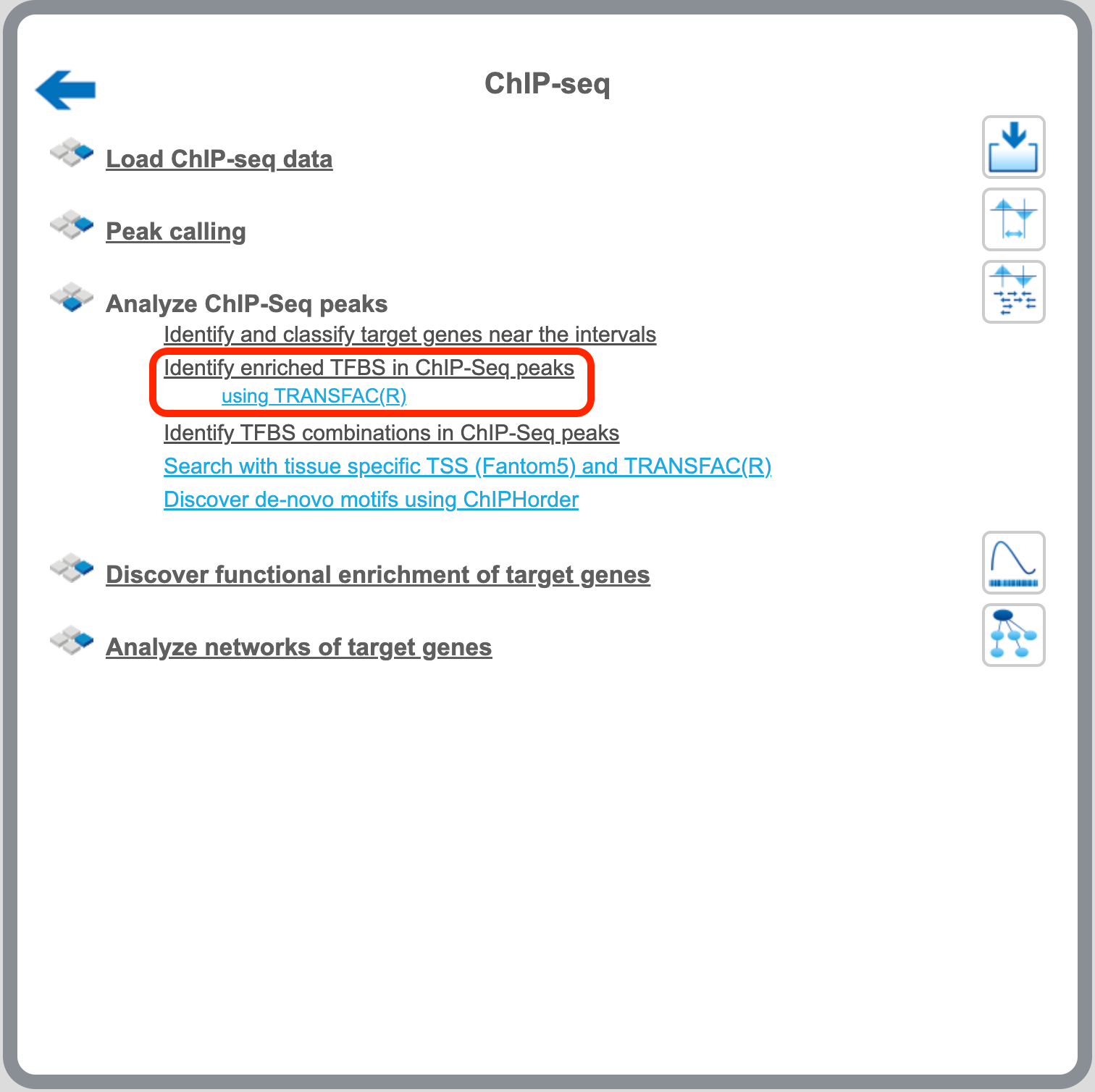
The workflow can be found under the section “Analyze ChIP-seq peaks” → Site search with TRANSFAC(R) → version 2.0 (Adjusted p-values).
To launch the workflow, follow these steps:
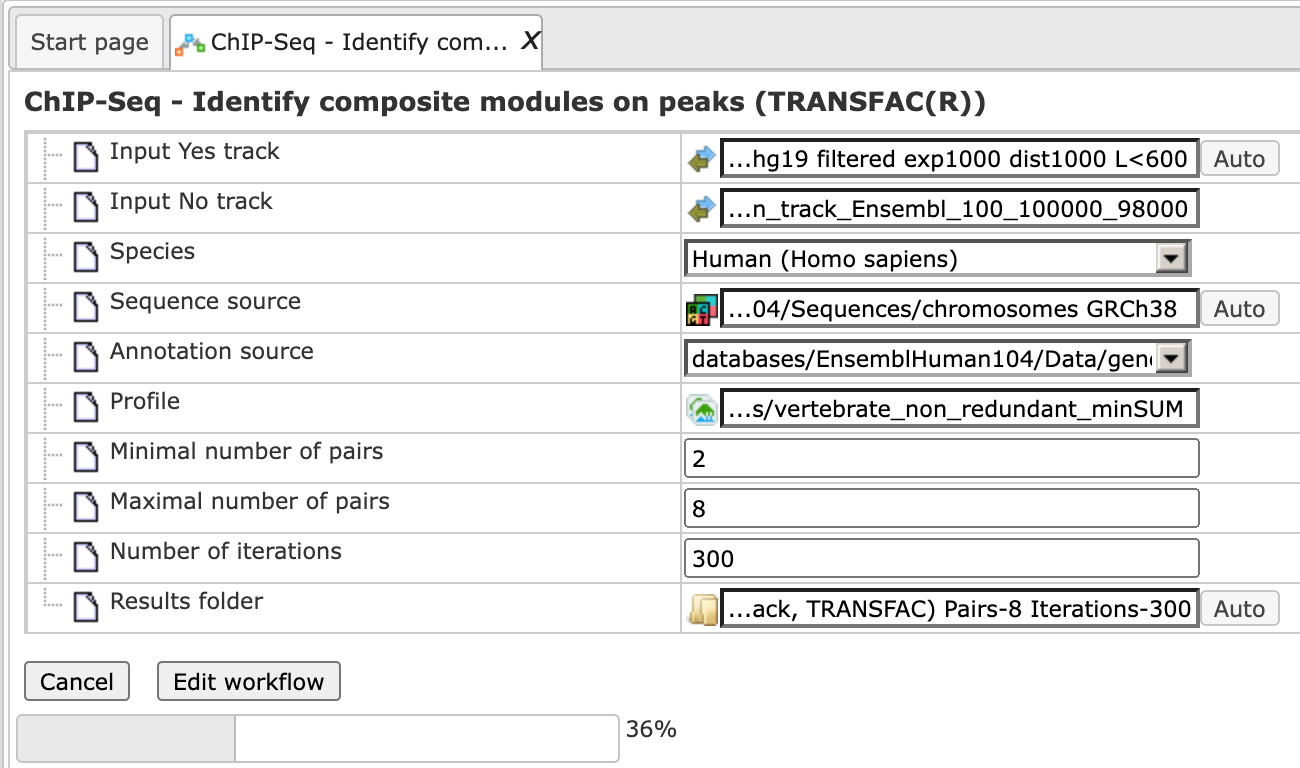
Step 1. Open the workflow input form from the Start page. It will open in the main Work Space and looks as shown below:
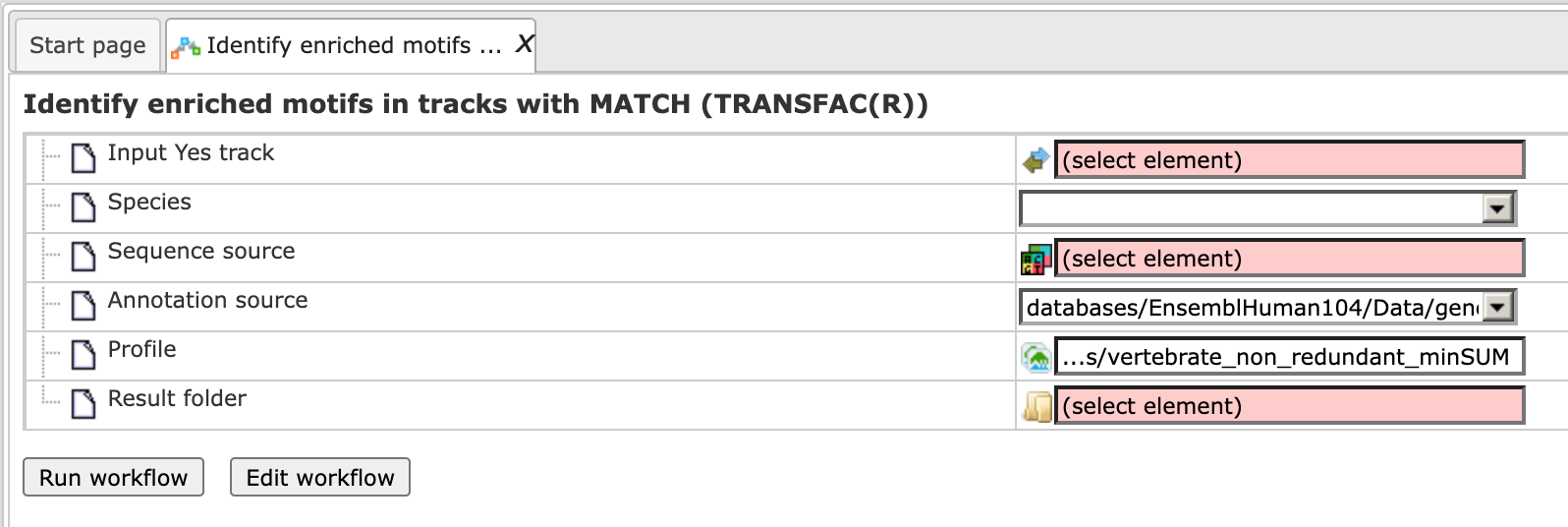
Step 2. Specify the input track in BED format in the field Input Yes
track.
The input Yes track contains peaks from your ChIP-seq study. To specify the Yes
track, you can drag & drop it from your project within the tree area.
Alternatively, you may click on the pink field “select element” and a new window
will open, where you select the input track. After having selected the track,
press the [Ok] button.
Step 3. Select the profile. This profile will be applied at the first part of the workflow for identification of the enriched motifs. The default profile is vertebrate_non_redundant_minSUM from the most recent [TRANSFAC® release]http://platform.genexplain.com/bioumlweb/#de=databases/TRANSFAC(R)2019.1/Data/profiles/ available.
Any other TRANSFAC® profile or user-specific profile can be selected. With a mouse click on the field Profile, a pop-up window will open, where a profile can be selected.
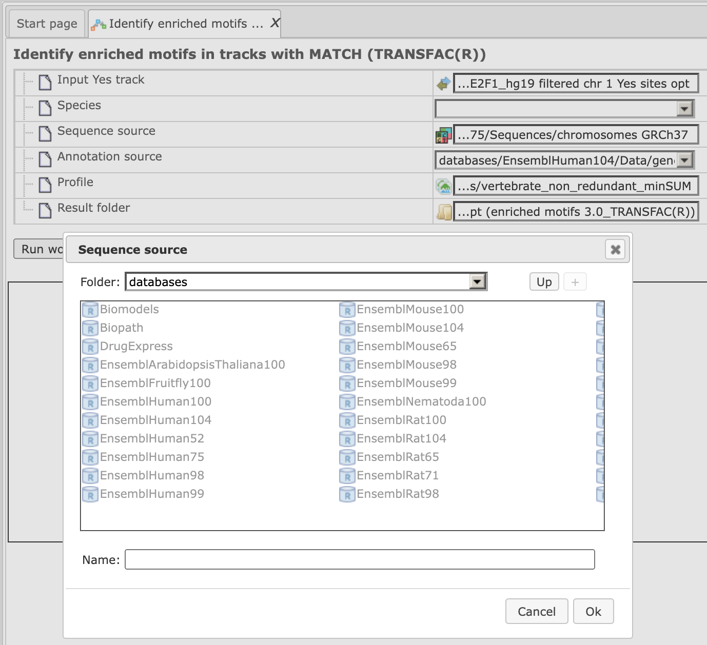
Step 4. Specify the sequence source from the drop-down menu. Several human, mouse and rat sequence builds are available in the platform, as shown below. By default, the most recent Ensembl human genome, hg19, is specified. Make sure you selected the sequence source (species and the genome build) that corresponds to your input set, to get correct and meaningful results.
Step 5. Specify the biological species of the input set in the field Species by selecting it from the drop-down menu.
Step 6. Select a filter for the coefficient of the MEALR method. The default filter is set as >0.125 to have 75% or more of true discovery rate, TDR. For 90% TDR, you can type 0.270 in this field and for 50% TDR - 0.05593. The filtered motifs are included in the output as enriched motifs. At the later step, PWMs corresponding to the enriched motifs are used to make a new profile.
Step 7. Define where the folder with the results should be located in your project tree. You can do so by clicking on the pink field “select element” in the field Result folder, and a new window will be opened, where you can select the location of the results folder and define its name.
Step 8. Press the [Run workflow] button.
Wait until the workflow is completed.
The Result folder contains several tables and three tracks; found here:
It is highlighted in blue in the figure below:
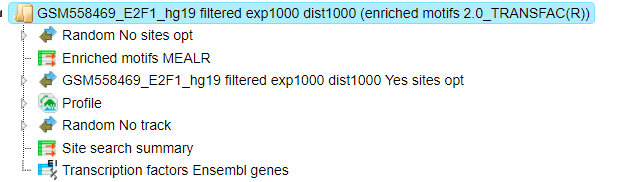
The tables Enriched motifs MEALR ( ) and Transcription factors
(
) and Transcription factors
( ) are opened automatically in the Work Space as soon as the workflow is
completed.
) are opened automatically in the Work Space as soon as the workflow is
completed.
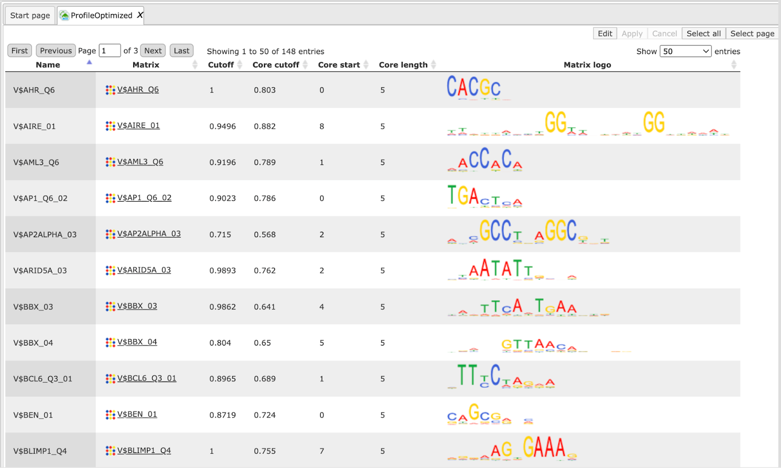
The table Enriched motifs MEALR includes enriched motifs in the Yes track versus the No track, filtered by the coefficient as specified.
Please note that by default only the matrices with a Coefficient >0.125 (75% True Discovery Rate) are included in this output table. These motifs can be interpreted as the best discriminating motifs between the Yes and NO sets.
The table Profile is opened automatically and is an input-specific profile, based on the filtered enriched motifs MEALR from the first part of the workflow.
This profile is an intermediate result of the workflow and is used further for Site search on gene set analysis in the second part of the workflow.
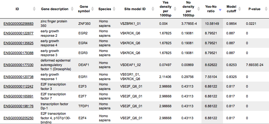
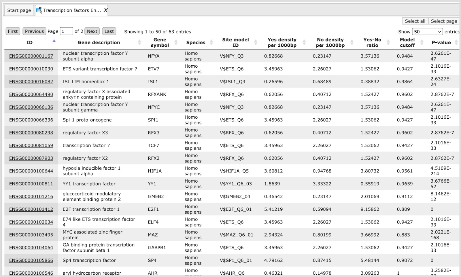
Table Transcription factors Ensembl:
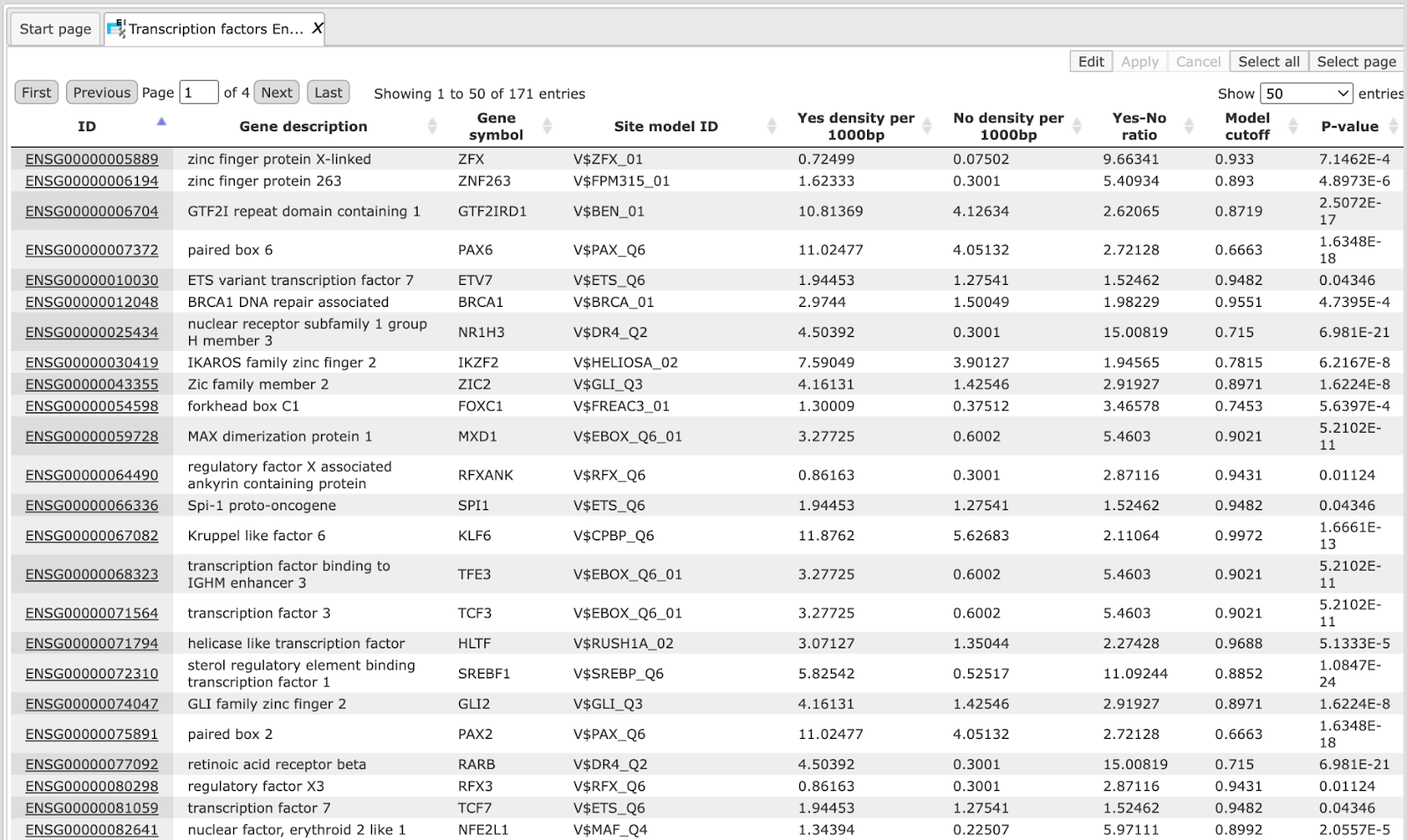
This table includes transcription factors (TFs) that are associated with the PWMs listed in the table Site search summary. Each row shows details for one TF, including its Ensembl gene ID (column ID), gene symbol, gene description and biological species of the corresponding TF (columns Gene description and Gene symbol). The column Site model ID shows the identifier of the PWM associated with this TF, and several further columns repeat information that is also shown in the table Site search summary.
Note This workflow is available together with a valid TRANSFAC® license. Please, feel free to ask for details (info@genexplain.com).
Version 1.2 (Classical)
Single interval list
This workflow helps to map putative TFBSs on peaks calculated from your
ChIP-seq data. Site search is done with the help of the TRANSFAC® library of
positional weight matrices, PWMs, using the pre-computed profile
vertebrate_non_redundant_minSUM.
The few steps to launch the workflow are described in the following.
Step 1. Open workflow input form from the Start page, it will be opened in the main Work Space and looks as it is shown below:
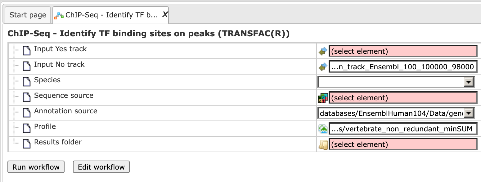
Step 2. Specify the input track in BED format in the field Input Yes
track.
The input Yes track contains peaks from your ChIP-seq study. To specify the Yes
track, you can drag & drop it from your project within the tree area.
Alternatively, you may click on the pink field “select element” and a new window
will open, where you select the input track. After having selected the track,
press the [Ok] button.
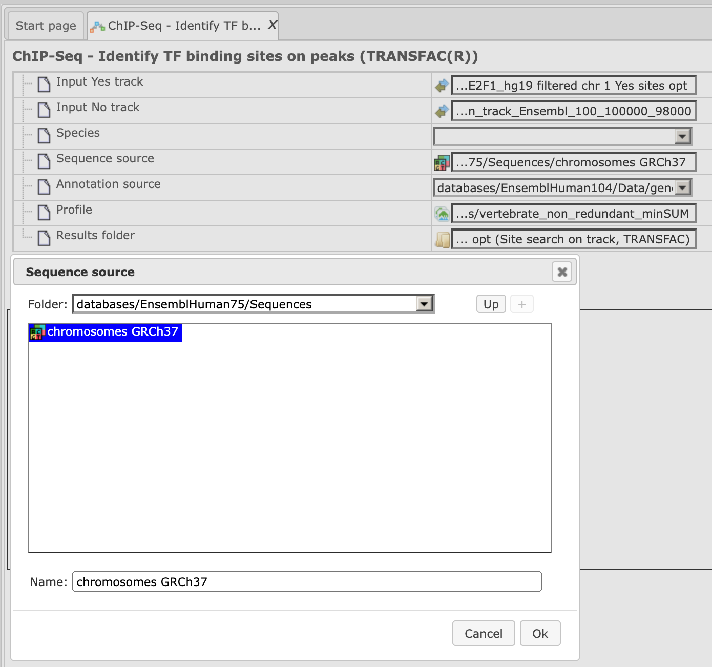
Step 3. Specify the sequence source from the drop-down menu. Several human, mouse and rat sequence builds are available in the platform, as shown below. By default, the most recent Ensembl human genome, hg19, is specified. Make sure you selected the sequence source (the genome build) that corresponds to your input set, to get correct and meaningful results.
Step 4. Specify the biological species of the input set in the field Species by selecting the required species from the drop-down menu.
Step 5. Specify No track in BED format in the field Input No track. Upon clicking on this field, a supplementary window will open, where you can select the No track from your project tree, or use one of our default No tracks for human, mouse or rat, respectively.
Step 6. Define where the folder with the results should be located in your project tree. You can do so by clicking on the pink field “select element” in the field Results folder, and a new window will be opened, where you can select the location of the results folder and define its name.
Step 7. Press the [Run workflow] button.
Ready!
Wait until the workflow is completed.
The results folder contains two tables and two tracks; for this example, let’s consider the results folder located under “Examples”. It is highlighted by blue in the figure below:
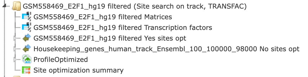
The tables Site optimization summary () and Transcription factors
() are opened automatically in the Work Space as soon as the workflow is
completed.
The table Site optimization summary includes the matrices the hits of which are over-represented in the Yes track versus the No track.
Please note that only the matrices with Yes-No ratio higher than 1 are included in this output table. The hits of these matrices can be interpreted as over-represented in the Yes set versus No set.
The table Site optimization summary shown below has been sorted by the values in the Yes-No ratio column.
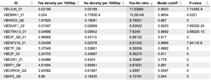
Each row summarizes the information for one PWM. For each selected matrix, the columns Yes density per 1000bp and No density per 1000bp show the number of matches normalized per 1000 bp length for the sequences in the input Yes set and input No set, respectively. The Column Yes-No ratio is the ratio of the first two columns. Only matrices with a Yes-No ratio higher than 1 are included in the summary table. The higher the Yes-No ratio, the higher is the enrichment of matches for the respective matrix in the Yes set. The matrix cutoff values as they are calculated by the program at the optimization step are shown in the column Model cutoff, and the last column shows the P-value of the corresponding event.
Table Transcription factors:
This table includes transcription factors (TFs) that are associated with the PWMs that are listed in the table Site optimization summary, and each row shows details for one TF, including its Ensembl gene ID (column ID), gene symbol, gene description and biological species of the corresponding TF (columns Gene description, Gene symbol, and Species). The column Site model ID shows the identifier of the PWM associated with this TF, and several further columns repeat information that is also shown in the table Site optimization summary.
Tracks “Yes sites opt” and “No sites opt” ( ).
).
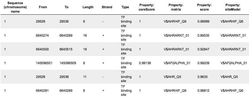
Each row presents details for each individual match for every PWM. Columns Sequence (chromosome) name, From, To, Length and Strand show the genomic location of the match including chromosome number, start and end positions, strand and length of the match, respectively. The column Type contains information about the type of the elements; in this case all matches are considered as “TF binding site”. Further columns keep information about PWM producing each match (column Property:matrix) as well as a score of the core (column Property:coreScore) and a score for the whole matrix (column Property:score). The column Property: siteModel contains an identifier for the site model, which is the matrix together with the cutoff applied (for details about these scores, please see Kel et al., Nucleic Acids Res. 31:3576-3579, 2003).
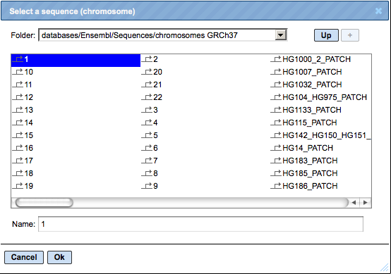
Tip. Further visualization of track files in the genome browser:
Having tracks “Yes sites opt” and “No sites opt” opened in the Work Space, the
menu button  can be applied to get a visualization. First, a supplementary window is opened where you can select one chromosome and press [Ok].<!–, as shown below.
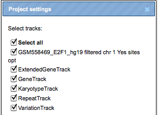
In the second pop-up window, you can select tracks that can be visualized together with your track, e.g. “Yes sites opt” (see above), and press [Ok].
 –>
–>
The resulting visualization, after applying the “zoom in” button, looks like it is shown below. Matches for different matrices are shown in colors, and the color schema can be customized.
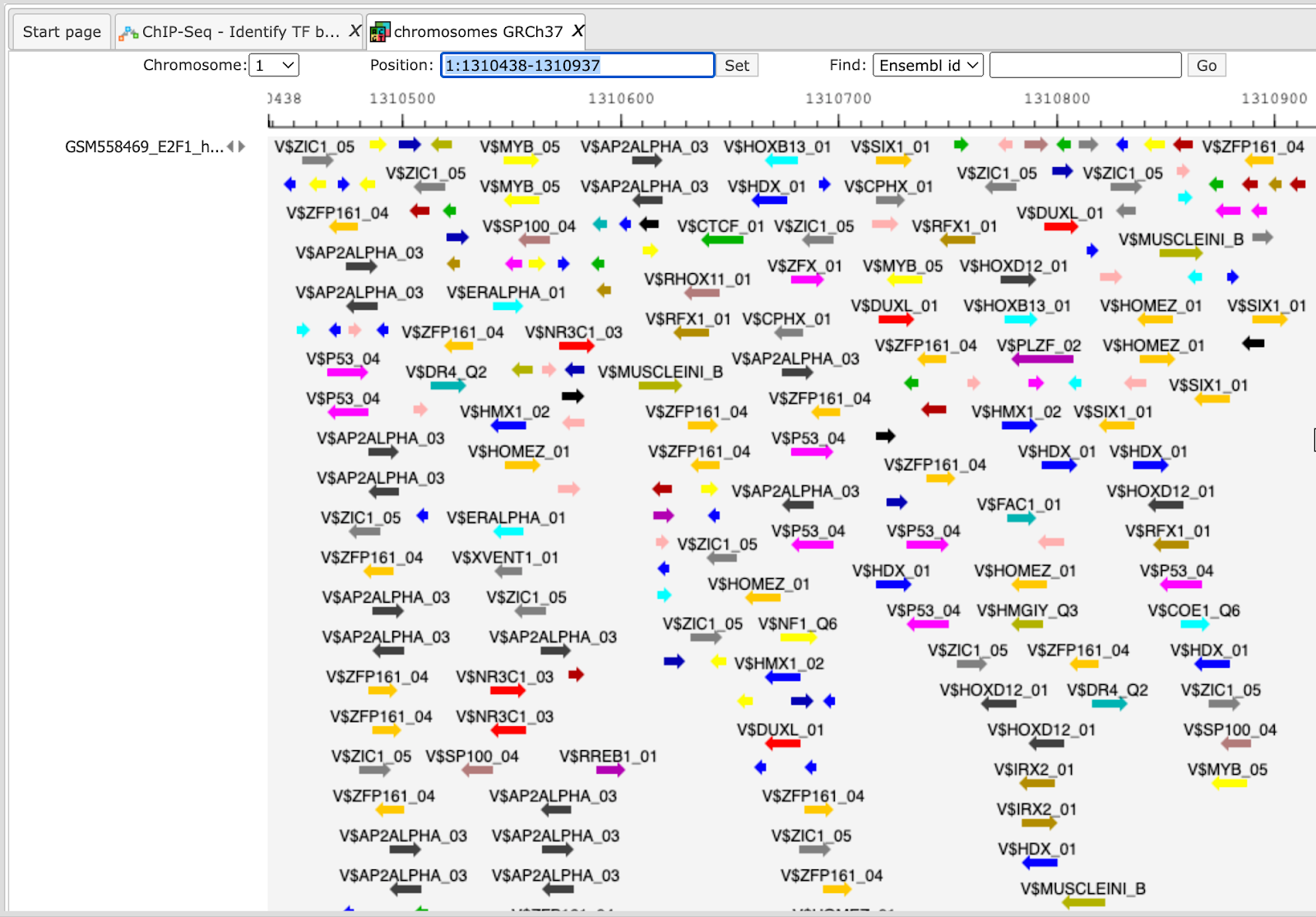
Such a view may help to visually co-localize information on different tracks, e.g. putative TFBS with variations, repeats and genes. In the figure above, the cursor shows position 29444, and two variations are located at this position. You can immediately recognize that these variations are located within particular putative binding sites in the intron region of the WASH7P gene.
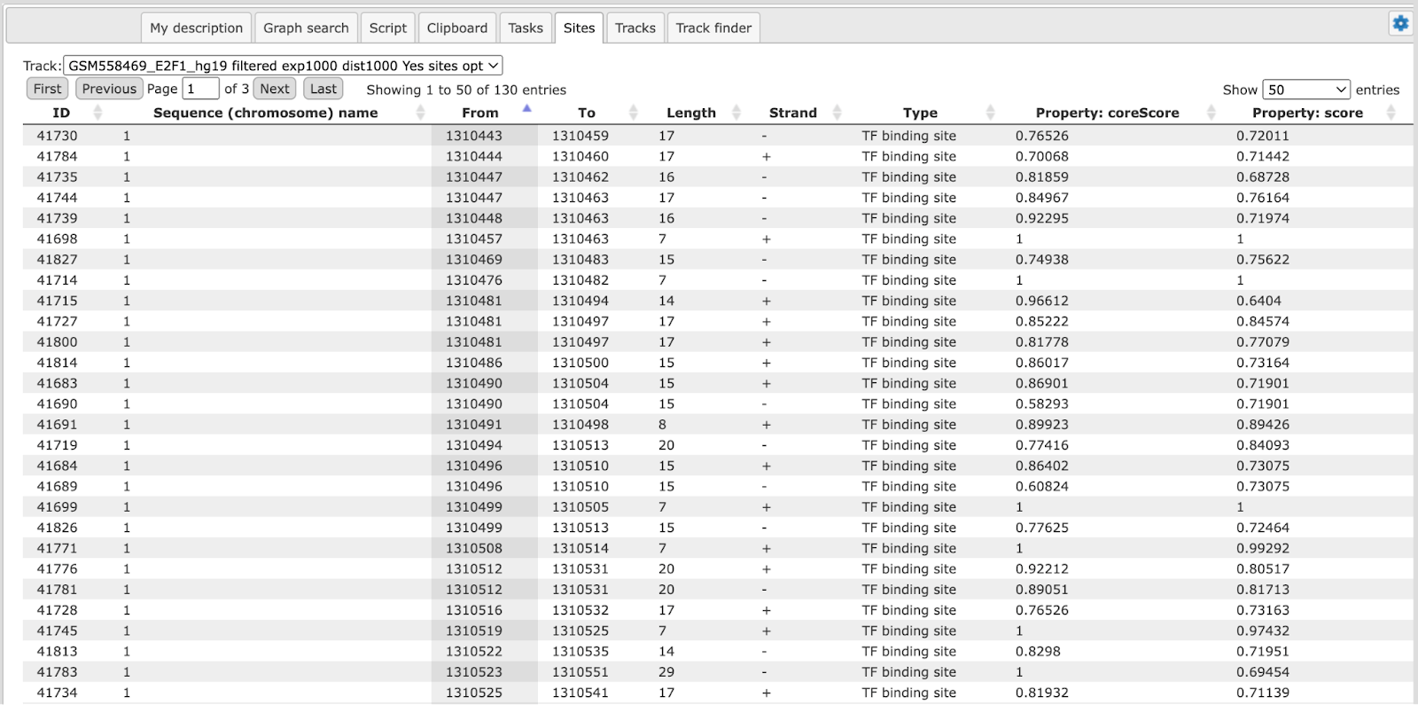
The same information is available not just as a picture, but also as a table under the tab “Sites” (shown below). For each element information is shown on chromosome, positions, length, strand, type of the track, and name of the element.
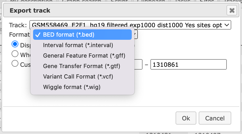
This table can be exported as a track, in several different formats including intervals, bed, wig, gff, gtf and more.
Note. This workflow is available together with a valid TRANSFAC® license.
Please, feel free to ask for details (info@genexplain.com).
Multiple interval sets
This workflow is designed to search for TFBSs in DNA sequences identified by the ChIP-seq approach, for multiple datasets.
In the field Input Yes tracks, several different tracks can be simultaneously submitted. The same background dataset, Input No track, is used for comparison with each of the submitted Yes tracks. The default No track corresponds to far upstream regions of the house keeping genes, where no functional TFBSs are expected.
The steps of this workflow for a single input Yes track are described in the previous section. In this workflow, the same steps are performed next time for the 2nd Yes track, and so on iteratively for each of the input Yes tracks.
This workflow helps to save time and effort, especially when you have several sets of ChIP-seq data, e.g. the peaks for a number of different TFs.
Note This workflow is available together with a valid TRANSFAC® license.
Please, feel free to ask for details (info@genexplain.com).
Search for composite modules with TRANSFAC®
This workflow finds pairs of TFBSs that discriminate between two tracks, the Yes and the No tracks. As the Yes track, the ChIP-seq peaks identified as binding profiles for particular transcription factors can be considered.
The ChIP-seq experimental technology is widely applied to a variety of biological problems, in particular to study genome-wide histone modification profiles, e.g. histone methylation and histone acetylation profiles. Correspondingly, the same workflow in the platform can be used to analyze histone modification profiles as well.
Here, let’s consider the results of the workflow application to find composite modules in the ChIP-seq peaks identified for in-vivo-bound fragments of transcription factor E2F1 in HeLa cells, published in Gene Expression Omnibus, GSM558469.
Input Yes track. The original track of genome-wide E2F1 binding fragments was filtered by the length shorter than 600 bp, which resulted in 249 fragments. This track of 249 fragments is used as the input Yes track. It can be found here:
Input No track. A track of the far upstream fragments of the human housekeeping genes located on chromosome 1 is taken as the No track found here:
The workflow input form is completed and the run is in progress:
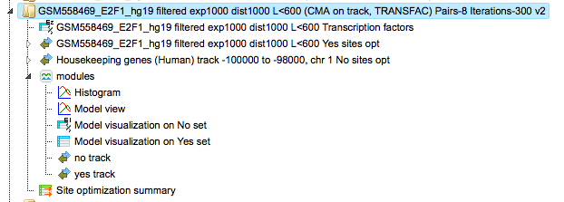
The resulting folder can be found under:
The table Site optimization summary ( ) contains those site models, here TRANSFAC® matrices, that are over-represented in the Yes track as compared to the No track.
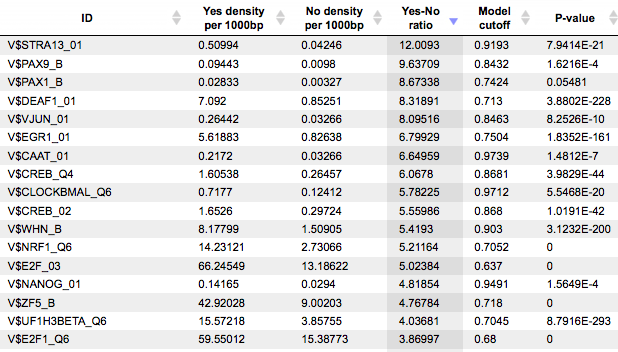
Each row of the table represents the result for one PWM from the input profile. Only those PWMs with Yes-No ratio >1 are included in the output. Upon sorting by the Yes-No ratio, matrices for E2F factors are among top 20 lines. Please note that the p-values of E2F matrices are extremely low, which demonstrates highest statistical significance of the results.
The Modules folder ( ). The composite module found contains two pairs, and we can see by exactly which site models (matrices) these pairs are formed as well as the statistical
parameters of the overall model.
). The composite module found contains two pairs, and we can see by exactly which site models (matrices) these pairs are formed as well as the statistical
parameters of the overall model.
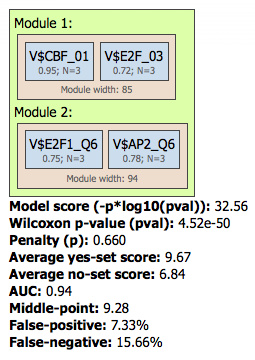
Both pairs contain matrices for E2F factors.
For more details on the individual output tables and tracks as well as for visualization of the identified composite modules in the genome browser please refer to the description of the method Identify composite modules.
Note This workflow is available together with a valid TRANSFAC® license.
Please, feel free to ask for details (info@genexplain.com).
Identify enriched motifs in tissue specific promoters
This workflow searches for enriched transcription factor binding sites (TFBSs) in a set of gene promoters versus a random promoter set. The input gene set is used to extract promoter regions by mapping it against the TSS locations defined in CAGE data in the Fantom5 (Nature 507:462–470) database . The overrepresented sites identified with the MEALR method are converted into a profile, which is used for a second round of site search, and ends up with the identification of transcription factors. To launch the workflow, open the workflow input form from the Start page:
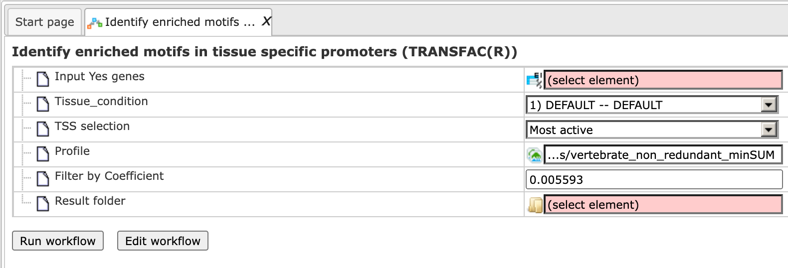
Step 1: To specify the Input Yes genes, you can drag & drop it from your project within the tree area. Alternatively, you may click on the pink field “select element” and a new window will open, where you select the input gene list. After having selected the list, press the [Ok] button.
For this example, all further steps are demonstrated with the following input set:
Step 2: Specify the biological species of the input set in the field Species by selecting the desired species from the drop-down menu.
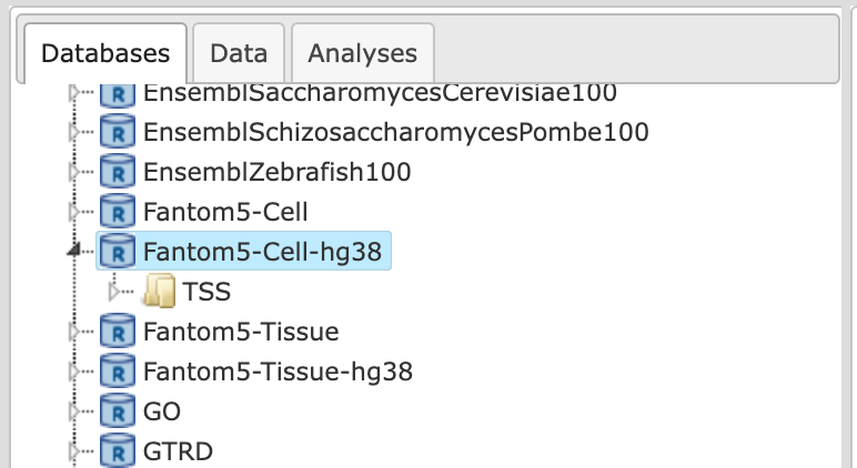
Step 3: Specify the Sequence source from the drop-down menu. Several human, mouse and rat sequence builds are available in the platform, as shown below. By default, the most recent Ensembl human genome, hg38, is specified. Make sure you select the sequence source (the genome build) that corresponds to your input set in order to get correct and meaningful results.
Step 4: Select the Tissue condition, select the tissue for which you want to create the promoter track from the drop-down menu.
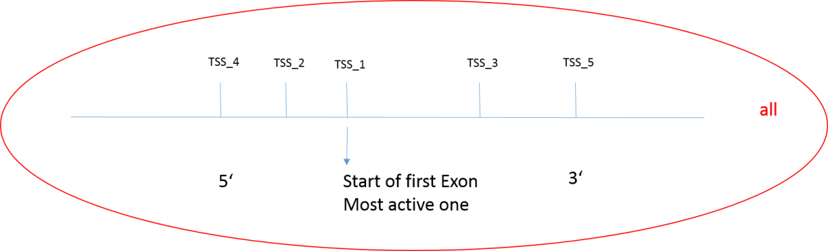
Step 5: The TSS selection should be performed if there are multiple transcription start sites. By default, the most active site is considered as TSS. You can select between most active, 5’ active, 3’ active and all (see below) from the drop-down menu.
Step 6: Define a TRANSFAC® profile. The default profile is vertebrate_non_redundant_minSUM. Any other TRANSFAC® profile or user-specific profile can be chosen. With a mouse click on the field Profile, a pop-up window will open, where a profile can be selected.
Step 7: Select a filter for the coefficient of the MEALR method. The default filter is set as >0.125 to have 75% or more of true discovery rate, TDR. For a 90% TDR, you can type 0.270 in this field and for 50% TDR - 0.05593. The filtered motifs are included in the output as enriched motifs. At the later step, PWMs corresponding to the enriched motifs are used to create a new profile.
Step 8: Define where the folder with the results should be located in your project tree. You can do so by clicking on the pink box (select element) in the field Results folder, and a new window will open, where you can select the location of the results folder and define its name.
Step 9: Press the [Run workflow] button. Wait until the workflow is completed, and take a look at the results.
Interpretation of results
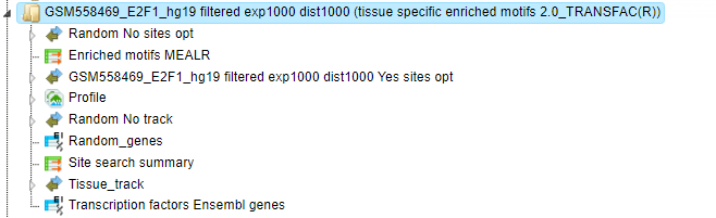
The result folder contains several files and one profile (collection of matrices):
Tracks
The input gene list is used to create tissue-specific promoter sequences as well as a random track. The random track includes 1000 random promoter sequences from the same sequence source as the input gene set. The resulting tracks are Tissue_track (from Input Yes genes) and Random_tissue_track.
Enriched motifs
The list of motifs, which were found during the first part of the workflow, and
were filtered by the coefficient > 0.125, can be found in the table
Enriched_motifs MEALR (). It contains those site models, here TRANSFAC® matrices, which are enriched in the Tissue_track in comparison with the Random_tissue_track. The example has
2 detected motifs with a coefficient > 0.125. The Profile contains the matrix
collection of converted and filtered site models. The table Transcription
factors Ensembl genes includes the corresponding 35 TFs from the second Site
search summary and is shown below:
Note This workflow is available together with valid TRANSFAC® and TRANSPATH® licenses. Please feel free to ask for details (info@genexplain.com).
Discover de-novo motifs using ChIPHorde and DiChIPHorde
ChIPHorde uses the fast heuristic of ChIPMunk, which is based on a greedy approach accompanied by bootstrapping, to search for multiple significant motifs in a given dataset using two independent filtering strategies. DiChIPHorde searches for di-nucleotide motifs that capture dependencies between neighboring motif positions.
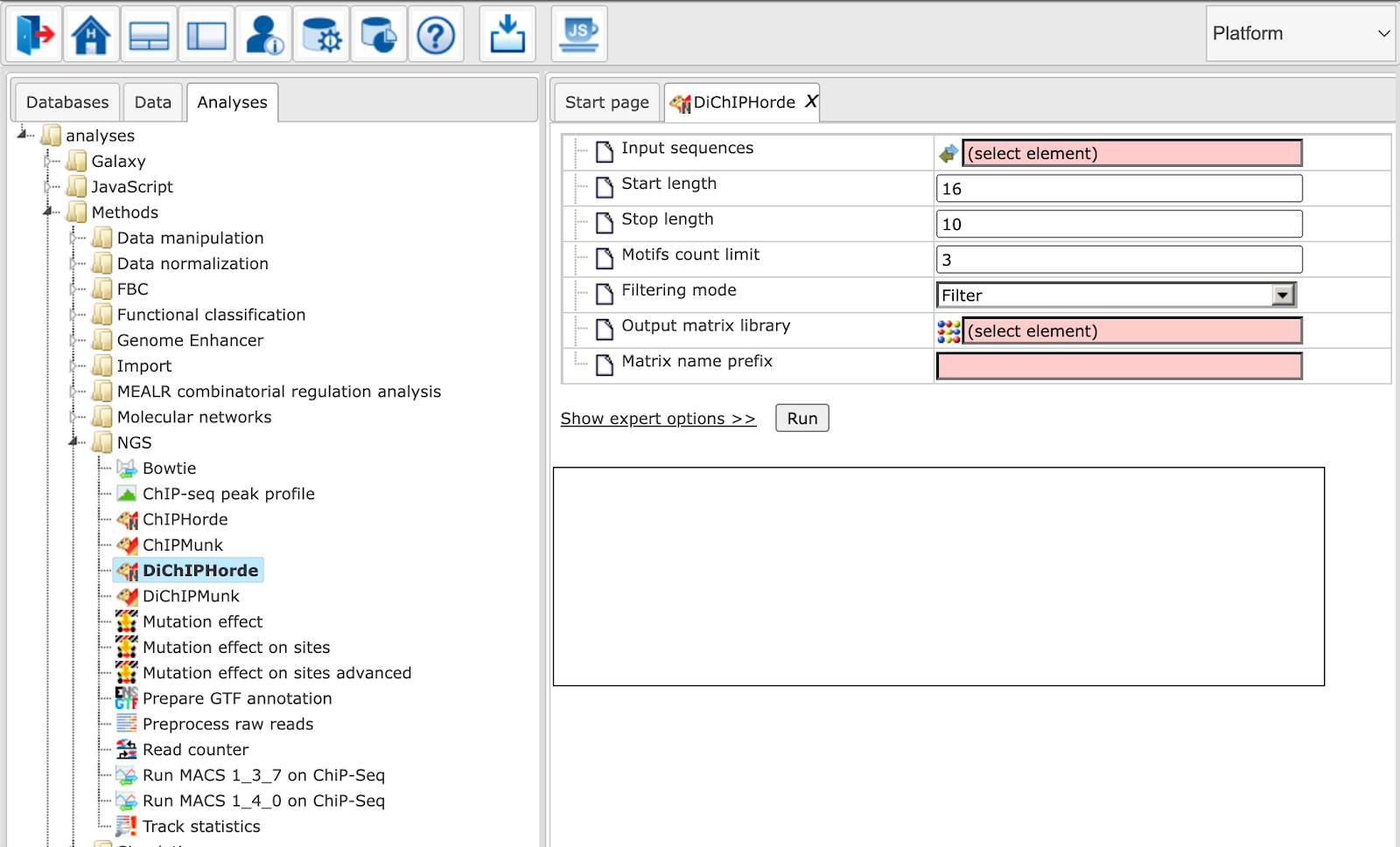
The image below shows the ChIPHorde interface. The input mask of DiChIPHorde features only slight differences as pointed out in the section describing input parameters.
The parameters are described in the following. For further details, please also refer to the ChIPMunk manual.
Input sequences: Track with input reads
Start length: Start length of the matrix
Stop length: Stop length of the matrix
Motifs count limit: Maximum number of motifs to discover
Filtering mode: Whether to mask polyN (”Mask”) or to drop entire sequence (”Filter”)
Number of threads (expert): Number of concurrent threads when processing
Step limit (expert): The number of bootstrapping runs. With a large data set or if unsure which computational time to expect, try a small number, e.g. 10.
Try limit (expert): This is a number of general optimization runs. For a random seeding this is equal to the number of seeds. As with “step limit”, apply the parameter with the size of your data set in mind. It is always advisable to test with a small number first.
Local background (expert): *DiChIPHorde only* If checked, local background estimation is used. Otherwise uniform background estimation is used
GC percent (expert): *ChIPHorde only* Relative GC content to be used as nucleotide background (0..1). Set to -1 to use the observed GC content.
ZOOPS factor (expert): Sets the preference for ZOOPS (Zero-or-one[-motif occurrences]-per-sequence) versus OOPS (Only-one-per-sequence) mode.
Motif shape (expert): The type of motif shape prior to use. The parameter corresponds a prior on the number of informative regions within the motif.
Use peak profiles (expert): Whether to apply peak profiles (if available).
Output matrix library: Path to the matrix library to be extended or created.
Matrix name prefix: Prefix for matrix names. It will be appended with a number.