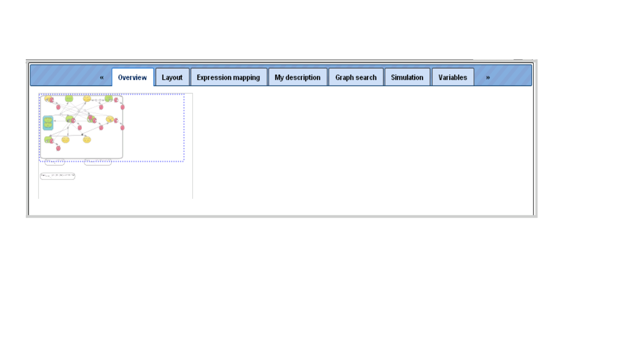
Operations field

In the Operations Field (D in the figure described in the section organization of genexplain platform ) a number of essential functions to operate the geneXplain platform are provided on a number of tabs. How many and which tabs are shown depends very much on the context.

Please note that not all tabs are always visible due to space constraints. In these cases, double arrowheads left and right of the tabs indicate that there are additional ones, reachable by clicking on these double arrowheads

The function of the individual tabs will be explained in more detail in those sections where their effect is part of a certain operation. In general, the icon initiates the corresponding activity within the Operations Field, whereas applies to the results generated in the Operations Field of the Work Space.

Changing the table structure in the Operations Field

Having opened a table in the Work Space, e.g. by double clicking on its name in the Tree Area, it is possible to edit its structure in the Operations Field under the tab Columns. For instance, if you have opened a table with data about Enrichment GO Molecular Mechanism (resulting from having run a GSEA), this field may look like this

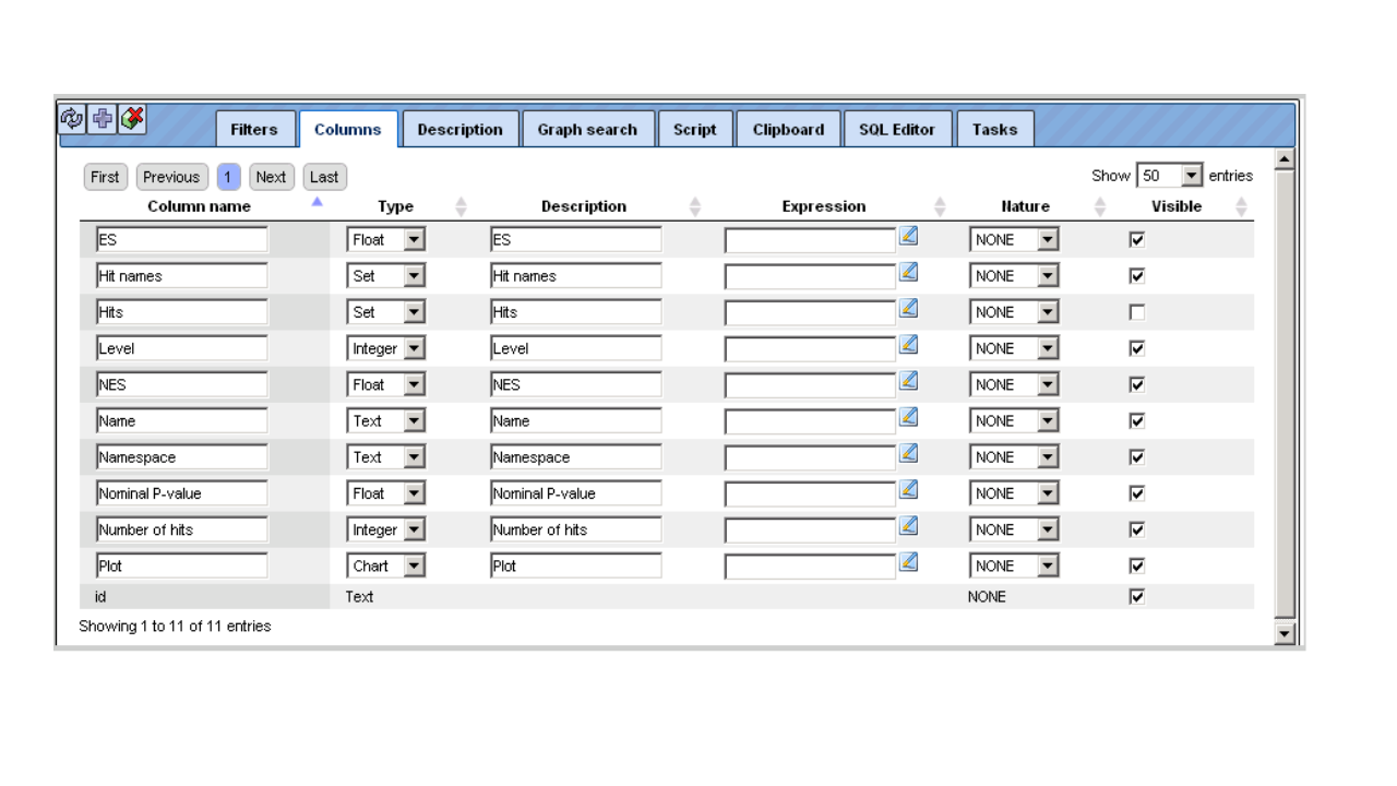
Recognizably, you can change the column headers, the data type in the column, or its (usually hidden) descriptions. You may add an Expression, which may be a mathematical formula, formulated in Java script; you find detailed explanations for this when you press the Edit key next to this field. In the last column, you can specify which columns are visible or shall be hidden (unmarking a column here does NOT delete it, it hides it from the currently displayed table).

If you hide a column by unmarking it, you have to refresh the Work Space by pressing the Refresh button in the control panel right on top of the Operations Field. Here, you can also add new () columns. Before removing a column with the button , you have to mark it by clicking somewhere in the background of the line specifying this column; the selected item will be highlighted in blue.

But be careful: Deleting it from the table will irrevocably erase the column including all its contents!

Changing the layout

Under the Layout tab, you can change the layout of the diagram. First, you can select one of the following layout schemes:

• Hierarchical layout (default)

• Orthogonal layout

• Force directed layout

• Cross cost grid layout

• Grid layout

When you have selected another layout type, you have to press the “Prepare layout” button (), showing the new layout at the right of the same window in the Operation Field. Pressing “Apply layout” transfer the new layout to the Work Space.

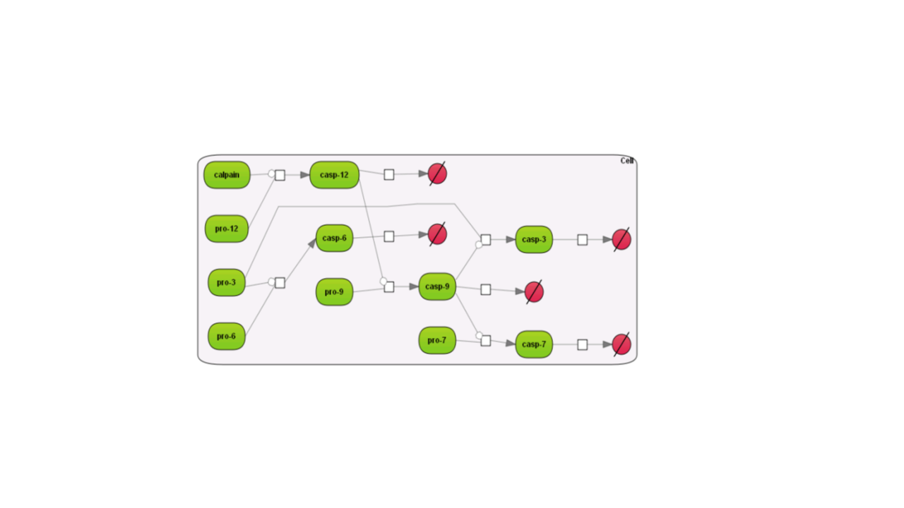
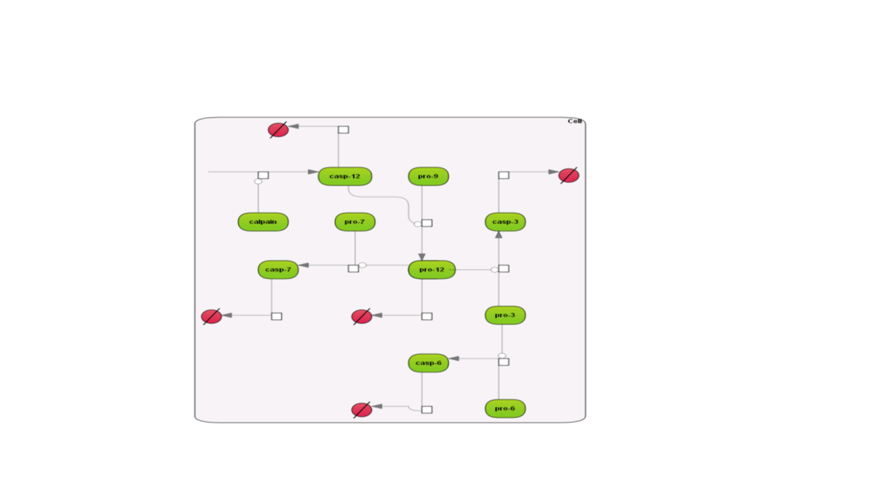
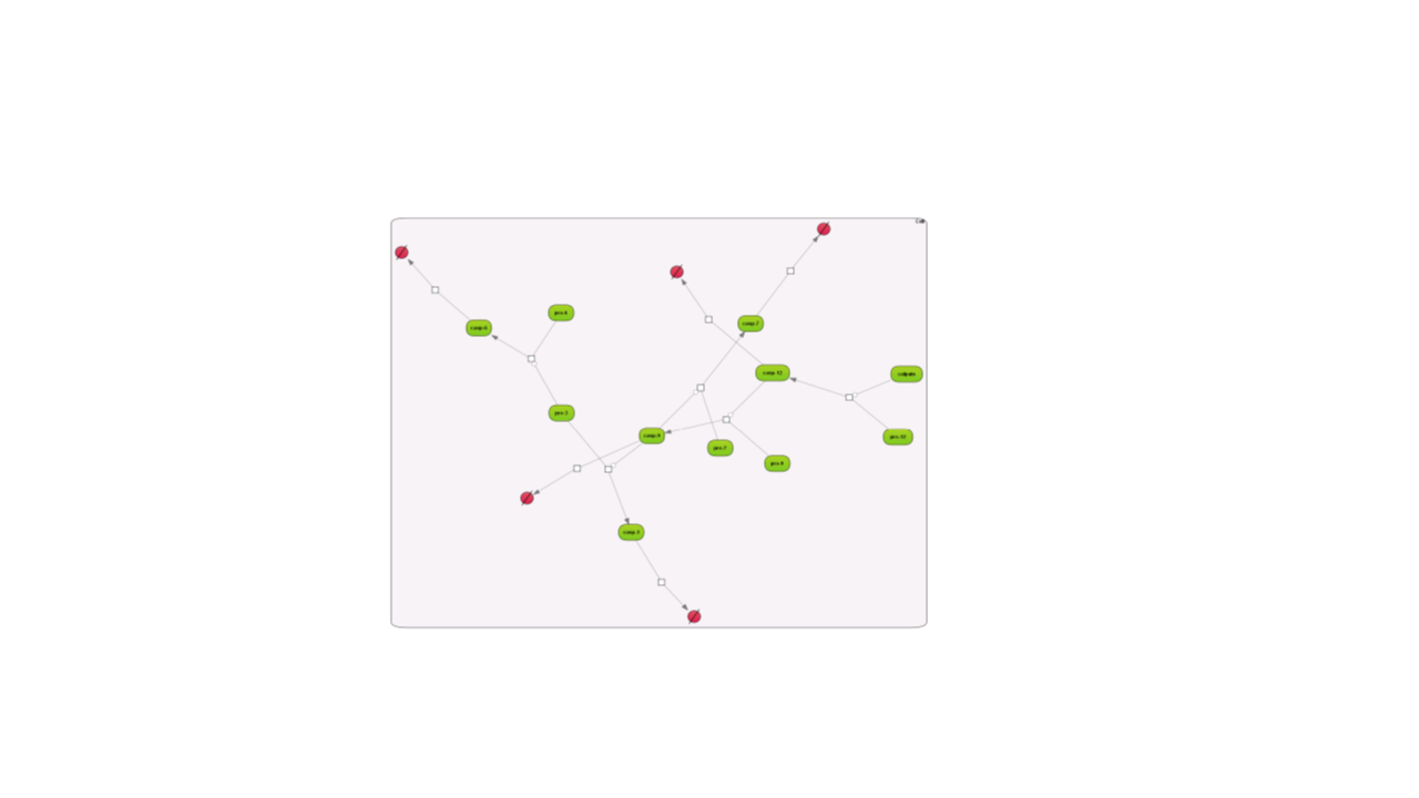
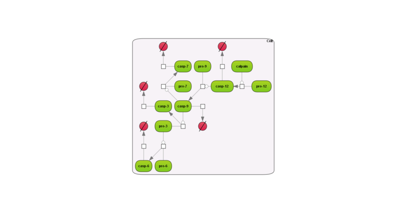
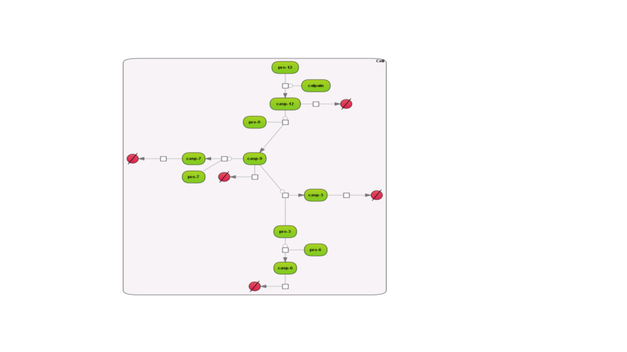
Here are examples how the different layouts look like; the example is the Caspase 12 pathway and has been taken from the database Integrated models (Int_casp12_module12):

Some of the re-layouting options may take considerable time. If you want to interrupt the process, press the “Stop layout” button.

The layout that has been applied to the Work Space can be further edited manually. A single click on a node (component or reaction node) highlights it; it can be shifted now by mouse movement, or can be deleted (right mouse button click opens a context menu with the option “Remove”). The results of this manual editing can be saved to the Operation Field so that they will be retained for the following work.

Please, be careful: changes in your own diagrams are automatically saved! You can even close the diagram in the Work Space, but still can undo your last changes with the Undo button (). After logout, all your changes will be automatically fixed.

Further editing of the layout schemes can be done by parameter settings in the Operation Field, Layout tab.

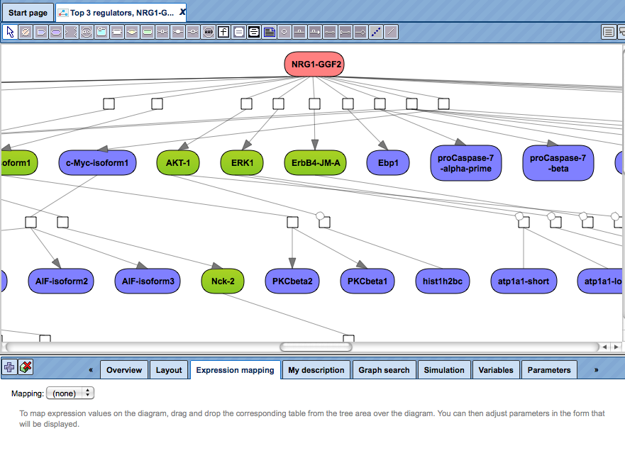
Expression Mapping

This function enables highlighting of up-regulated and down-regulated genes in the network diagrams.

The Expression mapping tab can be found in the Operations Field after having a network diagram opened in the work area. Initially, the expression mapping form is empty as shown in the figure below.

First, drag and drop the table with expression data from the Tree Area over the diagram. You might be interested to use the table with identified differentially expressed genes and calculated fold change values for expression mapping.

Important note. The format of the table with expression data that can be used depends on the format of the diagram. If the diagram was constructed based on the TRANSPATH® database, the format of the table to drag and drop should be “Proteins: Transpath peptides”, and the table should have the symbol

If the diagram was constructed based on the GeneWays database, the format of the table to drag and drop should be “Genes: Entrez”, and the table should have the symbol

Please check the format of the table with expression data before dragging and dropping it over the diagram, and if necessary, convert it to the required format with the function “Convert table” that can be found at the analyses/Methods/Data manipulation/Convert table.

After the table with expression data is dragged and dropped, the up- and down-regulated genes are automatically highlighted, and the expression mapping tab looks as shown below:

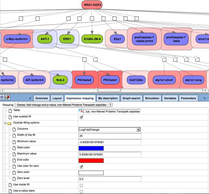
Let’s consider the main options/fields of the expression mapping form.

The default type of mapping is “outside fill”, and the corresponding check-box is checked, highlighted by the red oval below.

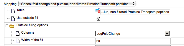
If the selected table contains a column LogFoldChange, this column is automatically chosen in the field “Columns”, highlighted by the green oval above. Other numerical columns in the selected table are available under the drop-down menu, and can be chosen instead of the default column to be applied for mapping expression data.

The fields Minimum value and Maximum value display the corresponding values of the selected column with expression data, (see highlighted red ovals in the figure below). These values are used to calculate the intensity of the colors for expression.

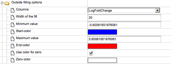
You can select colors to indicate up- and down-regulation by mouse click over the colored boxes, and the following toolbox will be displayed.

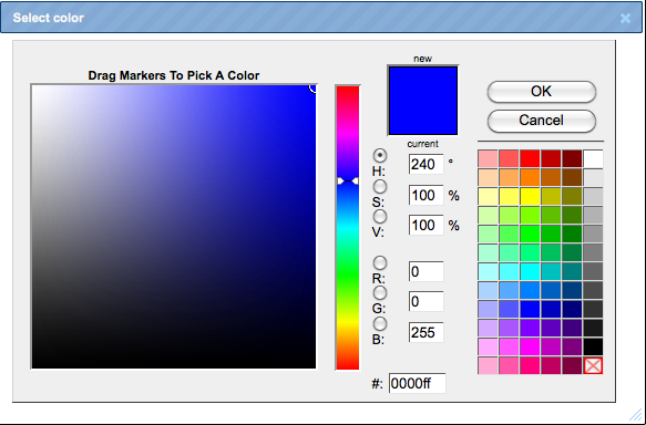
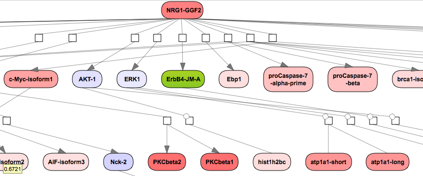
The expression values can be inferred by the color gradation. A more intensive color corresponds to a bigger fold change value whereas the lighter shade corresponds to a smaller fold change value. In this example all the up-regulated genes are shown with a color gradient from white to red whereas down-regulated genes are shown in with a color gradient from white to blue.

Check-in the box Use inside fill and check-out the box Use outside fill result in the following picture.

Graph Search

The “Graph search” option allows to extend diagrams already saved in the tree, e.g. to add interactions around the molecules in focus. Whenever a network diagram is opened in the Work Space, the “Graph search” tab can be found in the Operations Field as it is shown below.

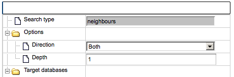
The gray fields in the graph search form cannot be edited. The user can change the search direction (upstream of the molecule in focus, or downstream, or both directions) and number of steps (depth) in the selected direction.

Graph search can be done in several iterations.

First iteration of a graph search.

To perform a graph search the following steps are recommended:

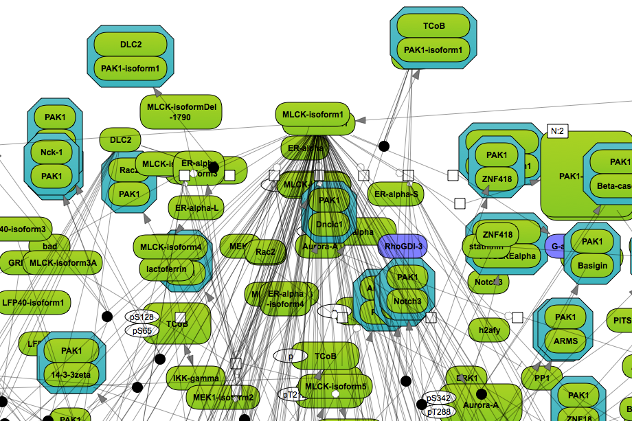
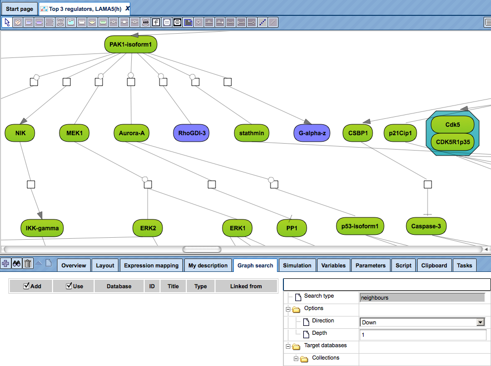
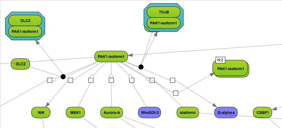
• Open a diagram in the Work Space and select one element (gene or protein or reaction) for which you want to perform search by mouse-clicking over that element. On the picture below, the molecule “PAK1-isoform1” has been selected, marked by the red oval.

• Use the button to add the selected molecule to the elements pane. The added element is marked by the blue oval on the picture below.

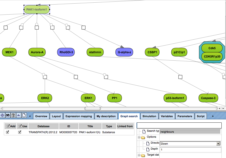
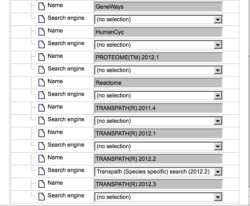
• Simultaneously, the database to search for additional interactions is automatically identified as the database based on which the network diagram is constructed. For the identified database the Search engine field is specified, marked by the blue oval on the picture below.

• Next, choose the direction and depth of search.

• Use

  to start the search. Once the search is finished you get the search results in the elements pane as shown in the screenshot below.

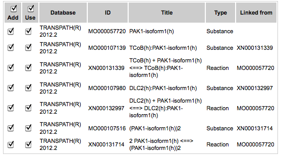
• When the Add box is checked, the corresponding molecules will be added to the diagram.
  The column with the check box Use means that selected molecules can be in turn used for searching, e.g. in the next search iteration. Direction of the search (up, down or both) and depth will be applied to the molecules with checked boxes in the Use column. By default, all boxes are checked. If you like to add to the diagram only a few molecules, you need to uncheck the others.

• In the next step, found molecules can be added to the current diagram by using the icon. By default all found molecules are checked. The user can uncheck some of the molecules in the column Add before adding to the diagram. Only the molecules checked in the column Add are added to the diagram. Here, all molecules are added, as shown on the picture below.

Now, the layout for the extended diagram can be specified, details of the layouts are described in Section “Changing the layout”.

If you would like to remove the search results and select another molecule, the delete button can be applied.

Second and next iterations of the graph search.

• Having several molecules in the element pane at the previous iteration of a graph search, the user can start searching again in the specified direction from these molecules.

• The user can uncheck some of the molecules in the column “Use” before starting the search again. Only the molecules checked-in in the column “Use” are used for the second search.

After the search is completed, all found molecules can be again added to the diagram, which may result in a picture, like shown below: