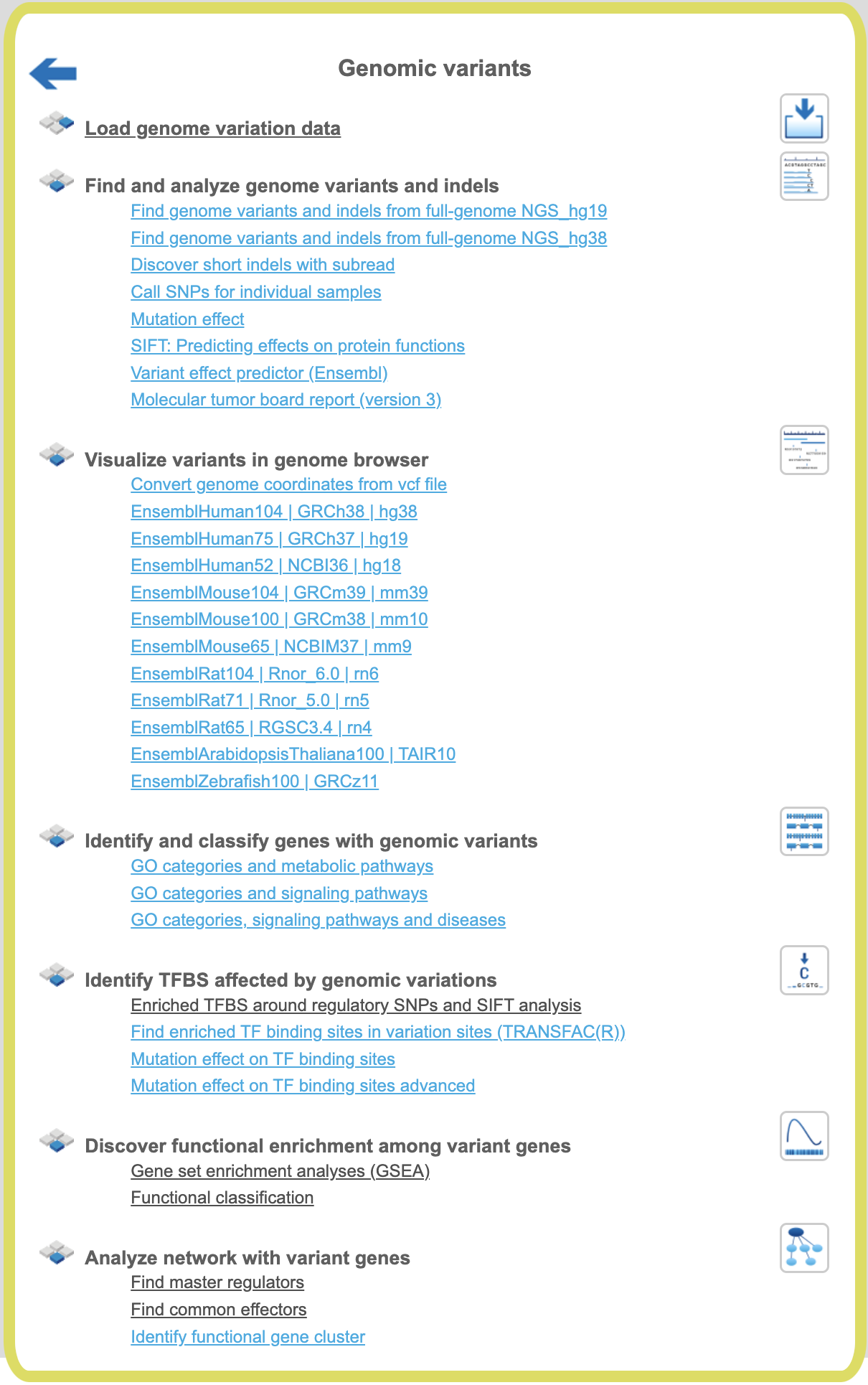
Genomic variants
Genomic variants can be uploaded to the platform in different formats. The files
uploaded in bed format are shown in the tree area as tracks ( ). Genomic variants can be also uploaded as a table, where the ID column contains standard SNP IDs (e.g. rs10010325). When imported into the platform,
the tables with this type of ID have a special icon (
). Genomic variants can be also uploaded as a table, where the ID column contains standard SNP IDs (e.g. rs10010325). When imported into the platform,
the tables with this type of ID have a special icon ( ) in the tree area. An example of such a table can be found in the Examples folder:
Find genome variants and indels from full-genome NGS
This workflow is based on a framework to discover genotype variations in full-genome NGS data by De Pristo et al., Nature Genetics 43:491-498, 2011. The process includes initial read mapping, local realignment around indels, base quality score recalibration, SNP discovery and genotyping to find all potential variants.
In the first part of the workflow the input sequences are mapped using the BWA tool (Galaxy). BWA is a fast light-weight tool that aligns relatively short sequences to a sequence database, such as the human reference genome (published by Li & Durbin, Bioinformatics 25:1754-1760, 2009).
The second part includes local realignment around indels, base quality score recalibration, SNP discovery and genotyping to find all potential variants. After the first part, and after identification of duplicates and covariates, the workflow creates a first output as a new BAM file. Then the recalibrated BAM file is used as an input for SNP discovery and genotyping to find all potential variants by GATK (Genome Analysis Toolkit).
To launch the workflow, follow these steps:
Step 1 Open the workflow input form from the Start page. It will open in the main Work Space and looks as shown below:
Step 2 Input the Forward and Reverse fastq files. You can either drag and drop or select the files from the Tree area. Example files are present here:
Step 3 Specify the OutputFolder location and name and press the button [Run workflow].
Results: Results are found in a folder can be accessed here:
In the first step the input fastq sequences are subjected to the BWA method from Illumina. BWA is a software package for mapping low-divergent sequences against a large reference genome, such as the human genome. It consists of three algorithms: BWA-backtrack, BWA-SW and BWA-MEM. The first algorithm is designed for Illumina sequence reads up to 100bp, while the other two algorithms are designed for longer sequences ranging from 70bp to 1Mbp. BWA-MEM and BWA-SW share similar features such as long-read support and split alignment, but BWA-MEM, which is the latest, is generally recommended for high-quality queries as it is faster and more accurate. BWA-MEM also has better performance than BWA-backtrack for 70-100bp Illumina reads.
In the next step the sorted files are subjected to the Mark Duplicates method.
This method removes duplicates. The purpose is to mitigate the effects of PCR amplification bias introduced during library construction. Two read pairs are considered duplicate if they align to the same genomic position. The resulting MarkDuplikates1.log file is stored in the log folder and the MarkDuplikates1.stat file is stored in the stat folder.
The next step is a local realignment. Read mapping algorithms operate on each read independently, locally realigning reads such that the number of mismatching bases is minimized across all reads. Output files are Realigner.log and TargetCreator.log in the log folder, ddup1.bam, Realigned.bam and realigner.intervals in the tmp folder.
The realigned BAM file is used again to remove duplicates (output MarkDuplicates2.log and MarkDuplicates2.stat), because realignment may change genomic positions of read pairs, after this step additional duplicates can be identified. The next step is a recalibration of base quality values. For each base in each read the method calculates various covariates (such as reported quality score, position in read, dinucleotide, read GC-content). Using these values it builds the model that predicts sequencing errors. Then it applies this model to calculate an empirical base quality score and overwrites the phred quality score in the read. Output is a new BAM file (Good.bam).
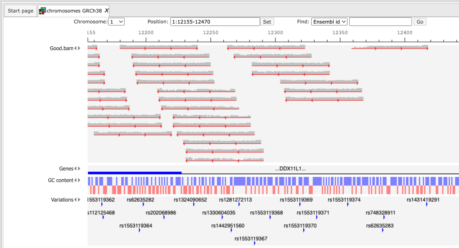
The user can view the Good.bam files in the genome browser by double-clicking on it. The browser shows each aligned read and also shows nucleotides mismatching between the reads and the reference genome sequence.
This file is used then for the unified GATK (Genome Analysis Toolkit) genotyper method to detect the SNP-indels. It generates a table in VCF format, which can be viewed either as a table or as a track in the genome browser (right mouse button click and select either “Open track” or “Open table”).
In the track visualization the information about each variation (either a base substitution or an indel) is shown in the info box when clicking on each variation.
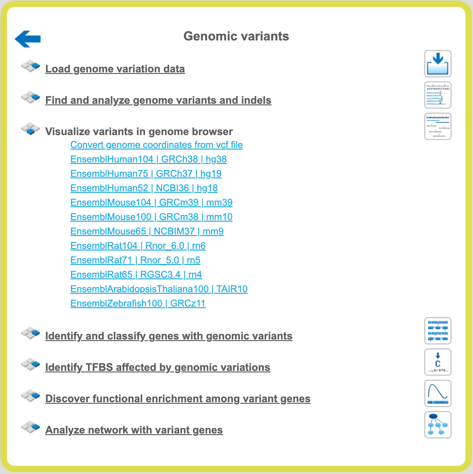
Visualize variants in genome browser
The genomic variants shown in the tree area as tracks () can be directly visualized in the genome browser. Tables with SNP IDs () should be first processed into the tracks. For this, you can apply the method called SNP matching ( );
);
For details please refer to the individual description of the method.
A mouse click on the links Human, Mouse or Rat immediately opens up a genome browser for the corresponding species in the work space, and the corresponding Ensembl database appears in the tree area.
Human
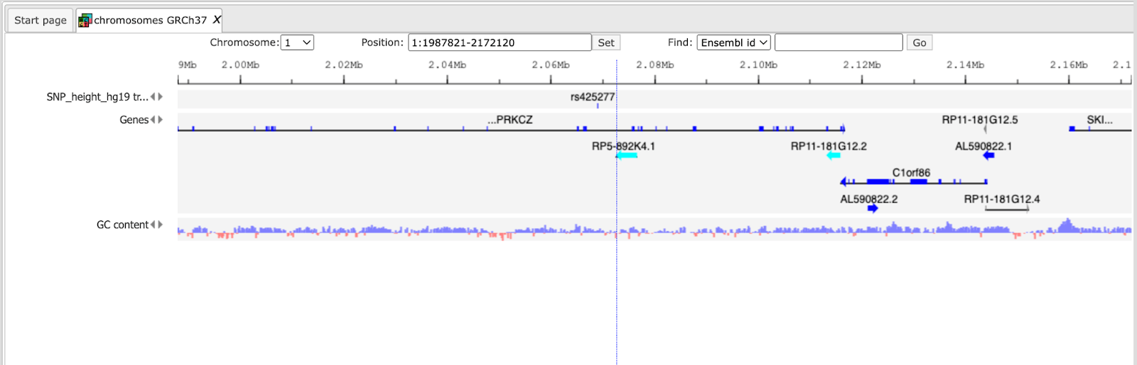
When Human is selected, the genome browser opens up the latest Ensembl build, hg38 chromosomes GRCh38.
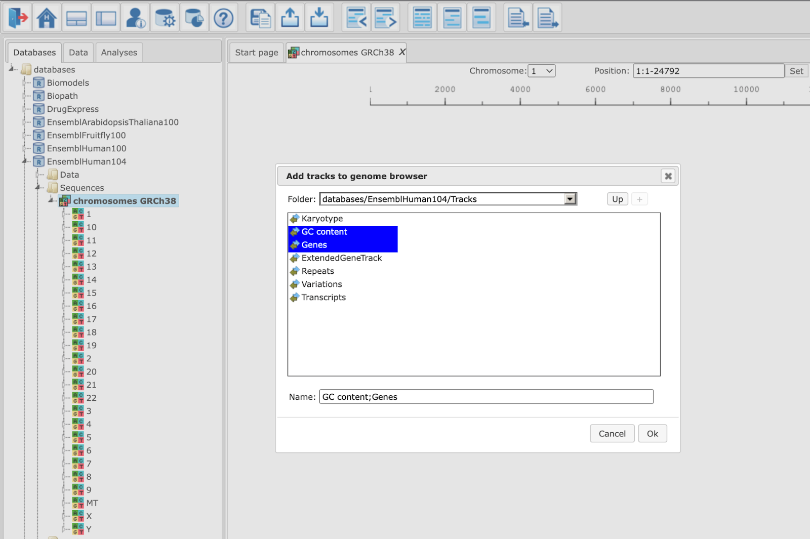
In the pop-up window Add tracks to genome browser you can select which tracks among those available in Ensembl should be opened together with your track of the genomic variants. Two tracks are selected by default, GC-content and Genes. When the selection is ready, push the [Ok] to get the following view:
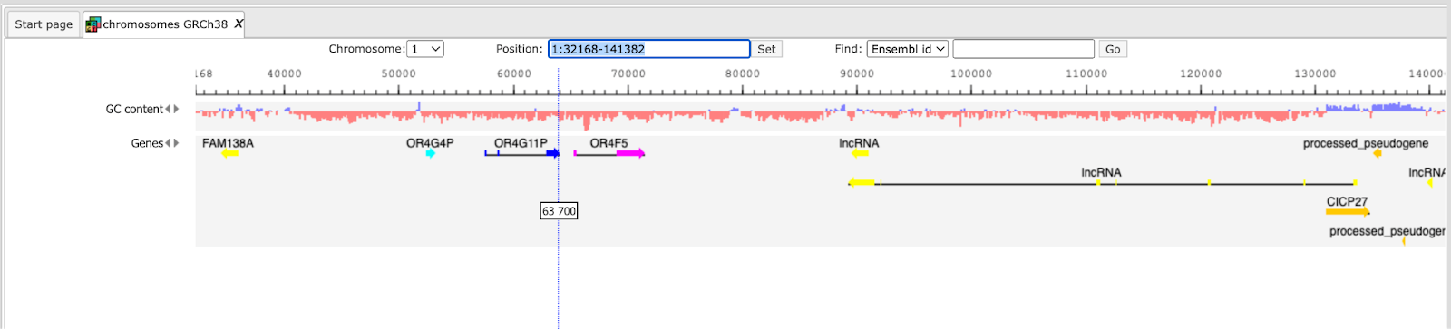
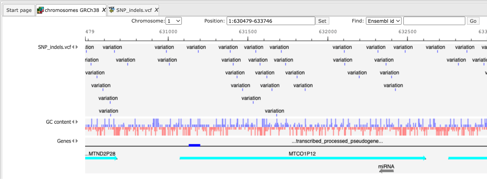
Now you can drag & drop your track with the genomic variants on the genome browser to add it to the default tracks. As an example, the following track is shown here, in the screenshot below:
For further details regarding visualizations, please refer to the basic operations with tracks
Mouse
When Mouse is selected, the genome browser opens up the latest Ensembl build for mouse, mm39 chromosomes GRCm39
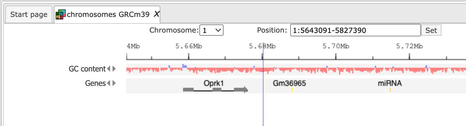
The further steps of the visualization are similar to the human tracks.
Rat
When Rat is selected, the genome browser opens up the latest Ensembl build for rat, rn6 chromosomes Rnor_6.0
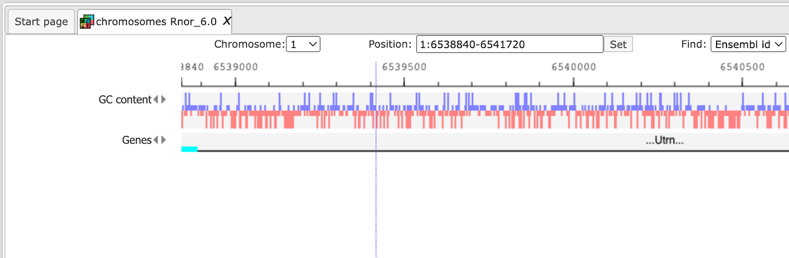
The further steps of the visualization are similar to the human tracks.
Identify and classify genes with genomic variants
Genomic variants are represented in the same format as genome intervals or ChIP-seq peaks, i.e. with their absolute chromosomal positional locations. Therefore, please apply correspondingly the workflows explained in detail under Epigenomics and Chip_Seq sections.
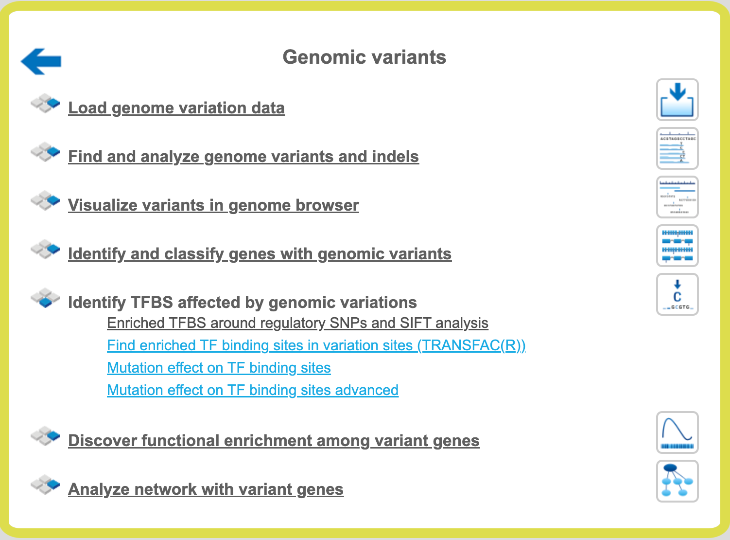
Identify TFBS affected by genomic variations
Enriched TF sites around regulatory SNPs and SIFT analysis
Analysis with TRANSFAC®
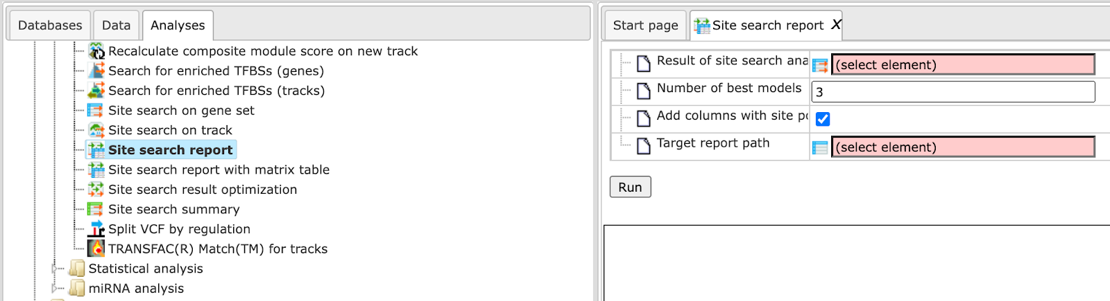
The input form of this workflow, when opened from the Start page, is the following:
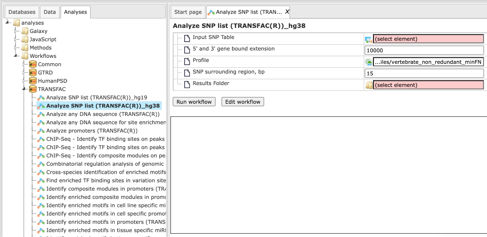
Step 1 Specify an input table in the field Input SNP table. A table
with standard SNP IDs in the format like rs10010325 can be used as an input.
The tables with this type of IDs have a special icon () in the tree area. In this example the following input table with 180 SNPs is used:
Step 2 Specify the region around each SNP in the field 5’ and 3’ gene bound extension. By default this region is 10000 bp long. Genes located within the region of 10000 bp around each SNP in the input list will be considered as SNP target genes.
Step 3 Specify a TRANSFAC® profile in the field Profile. The workflow uses the default profile vertebrate_non_redundant_minFN from the TRANSFAC® library, but another TRANSFAC profile can be chosen as needed.
Step 4 Specify the region around each SNP that will be analyzed for potential TFBSs in the field SNP surrounding region. The default length of this region is 30 bp on each flank.
Step 5 Select a species corresponding to your input table from the drop-down menu in the field Species.
Step 6 Specify the path to store the results and the name of the output folder in the field Results folder.
Step 7 Having filled the input form, launch the analysis with the [Run] button. Wait till the workflow is completed.
Results
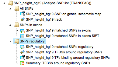
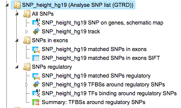
The output is a result folder with three subfolders named all SNPs, SNPs in exons and SNPs regulatory, respectively, containing all resulting tables and tracks:
The results shown here can be found here:
Subfolder All SNPs
This folder includes one gene table and one track.
The table SNPs on genes, schematic map ( ) contains all genes that were identified in the region of 10000 bp on both flanks around each SNP, in this example 119 genes.
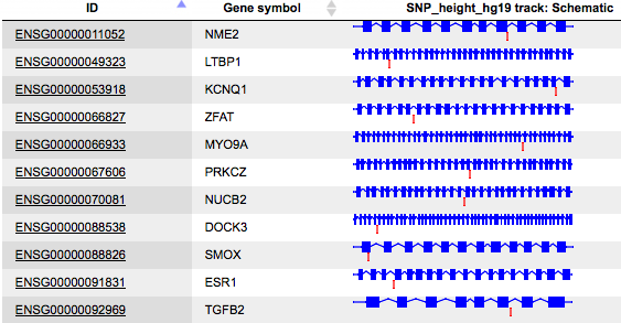
Each row of this table corresponds to one gene; the column ID presents Ensembl gene IDs, and HGNC gene symbols are listed in the column Gene symbol. The title of the last column Schematic also contains the name of the input table. This column represents a schematic view for each gene, where blue boxes correspond to exons, and the lines between exons symbolize introns, drawn in logarithmic scale. SNPs are shown by vertical red lines. This schema provides an overview of SNP location within genes.
A track () represents the results of the SNP mapping to genomic positions. In this
example, out of 180 input SNPs 148 were mapped to the genome, and for them the
following information is shown:
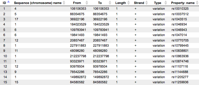
For each SNP the tabulated view of the track contains information about chromosomal location, absolute positions, length, and strand. In the column Type the value variation is shown for all SNPs, and in the column Property: name SNP IDs are shown.
Subfolder SNPs in exons
This folder includes two tables, both present information for those SNPs that are located in exons. In our example, 19 out of 148 SNPs mapped to the genome are located in exons.
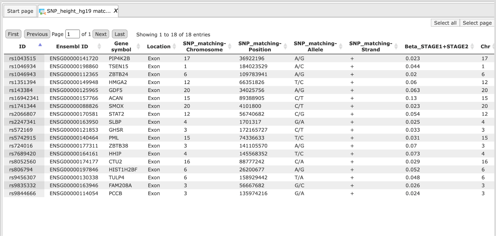
One of the tables contains standard SNP IDs in the ID column, and has the
same icon as the input SNP table ().
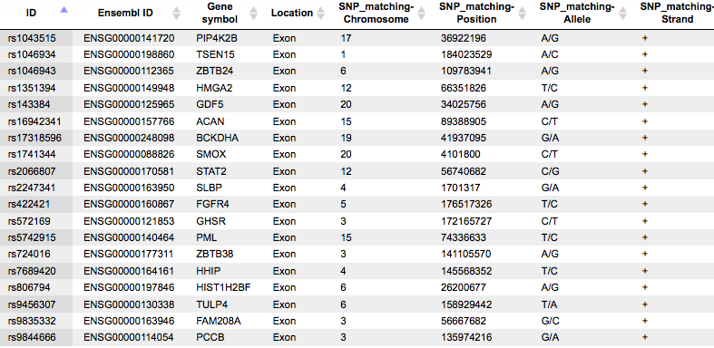
This table contains general information about SNPs that are located in exons. Each row in this table corresponds to one SNP. The columns Ensembl ID and Gene symbol refer to the gene in which this particular SNP is located. The column Location confirms that all SNPs are located in exons. The absolute genomic positions of the SNPs are shown in the columns SNP_matching-Chromosome, SNP_matching-Position and SNP_matching-Strand. The column SNP_matching-Allele shows which nucleotide exactly varies at the listed position.
If your input SNP table contains more columns in addition to IDs, all these columns will be preserved and will be added to the right side of this table.
The other table in this subfolder results from the SIFT analysis, and is represented by an icon for a general table.
SIFT is a widely accepted method to check whether a particular variation is synonymous or non-synonymous, and in case of a non-synonymous variation whether it is damaging or tolerated. More details about SIFT can be found under http://sift.jcvi.org/www/SIFT_help.html.
This table also has 19 rows according to the number of SNPs identified in exons. There are many columns in this table, we will consider the most important ones in the following.
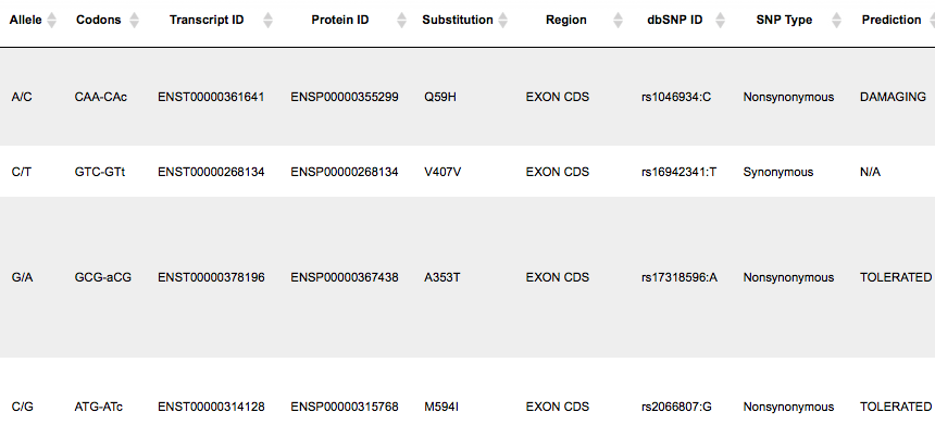
The columns Codons and Substitution show which nucleotide in a codon varies and which amino acid is substituted by which. The column SNP Type shows if it is a synonymous or a non-synonymous variation, and in case of non-synonymous variations the column Prediction shows if it is damaging or tolerated. An extension of this table to its right side is shown below, starting with the column Prediction:
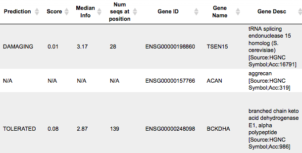
The columns Gene ID, Gene Name, Gene Desc show information about which genes and gene products are affected and might be even damaged by a given variation.
Subfolder SNPs regulatory
This subfolder contains three tables and one track.
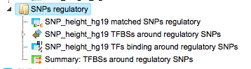
In this example, 129 out of 148 SNPs mapped to the genome are located in introns or gene flanking regions. The table contains standard SNP IDs in the ID column, and has the same icon as the input SNP table, and as the table with SNPs in exons. The structure of the latter was described above in detail, under the subheading Subfolder SNPs in exons.
The other two tables and one track in this subfolder present the results of the TFBS search in the SNP surrounding regions.
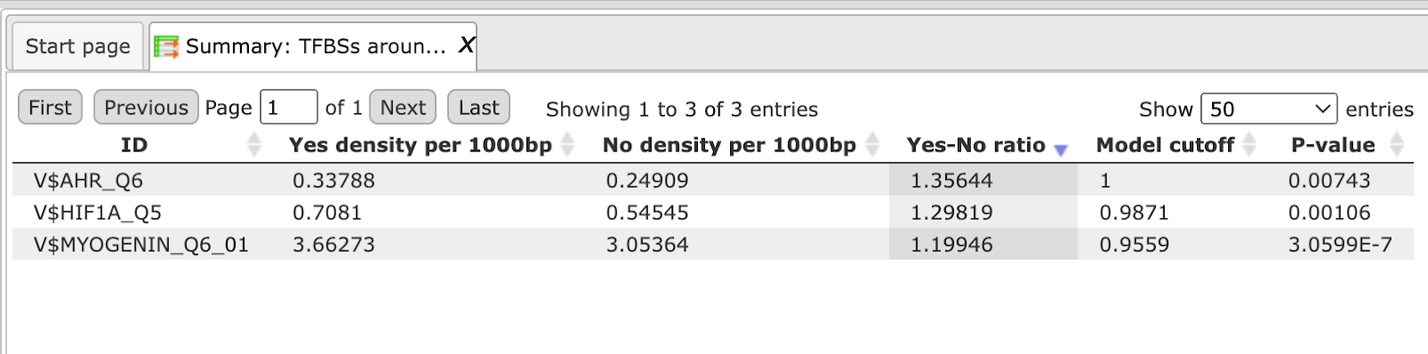
The table Summary: TFBSs around regulatory SNPs ( ) shown below has been sorted by the values in the Yes-No ratio column.
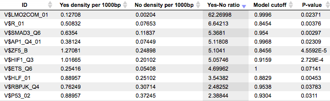
Each row summarizes the information for one PWM. The columns Yes density per 1000bp and No density per 1000bp show the number of matches normalized per 1000 bp length for the sequences around SNPs and in the sequences around random genomic positions, respectively. The column Yes-No ratio is the ratio of the first two columns. Only matrices with a Yes-No ratio higher than 1 are included in the Summary table. The higher the Yes-No ratio, the higher the enrichment of matches is for the respective matrix in the sequences around regulatory SNPs. The matrix cutoff values calculated by the program at the optimization step are shown in the column Model cutoff, and the last column shows the P-value of the corresponding event.
The table TFs binding around regulatory SNPs ()
includes transcription factors (TFs) that are associated with the PWMs listed
in the table above, and each row shows details for one TF, including its Ensembl
gene ID (column ID), gene symbol, gene description of the corresponding TF
(columns Gene description, Gene symbol). The column Site model ID
shows the identifier of the PWM associated with this TF, and several further
columns repeat information that is also shown in the table above.
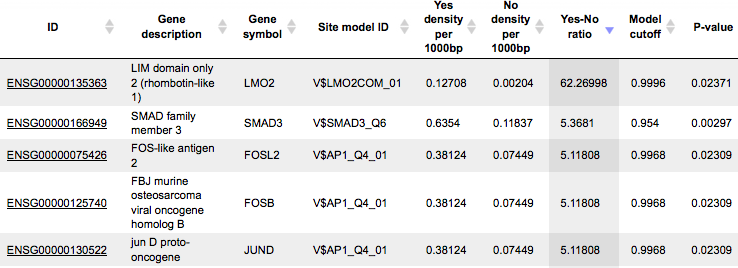
These TFs are suggested to have their binding sites in close proximity or even overlapping with SNPs, and their binding might be affected by a given SNP.
The track TFBSs around regulatory SNPs ( ) gives information about the genomic positions of the identified TFBSs.
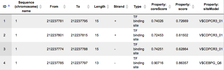
Each row presents details for an individual TFBS. The columns Sequence (chromosome) name, From, To, Length and Strand show the genomic location of the match including chromosome number, start and end positions, strand, and length of the match. The column Type contains information about the type of the elements; in this case all matches are assigned the type TF binding site. Further columns keep information about the site model producing each match (column Property:siteModel) as well as a score of the core (column Property:coreScore), and a score for the whole site model (column Property:score).
Tip When having tracks opened in the Work Space, the menu button ( ) on the top panel can be applied to visualize it. A supplementary window Add tracks to genome browser will open. Here you can select tracks that can be visualized together with your track (shown below).
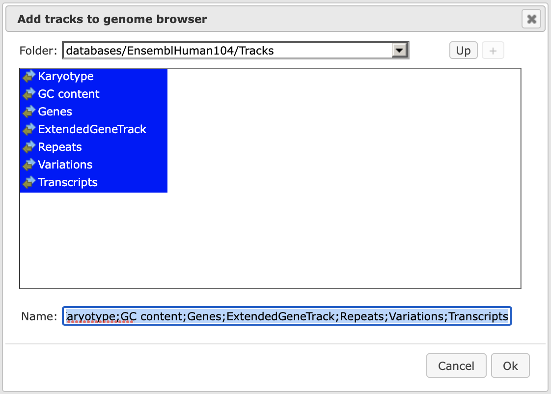
After pressing [Ok] you will get the picture shown below with your track in focus at the top position.
A number of options are available to navigate the browser and get the desired view. You can use several buttons at the top panel to zoom in and out, and to shift the visible part of the map left or right.
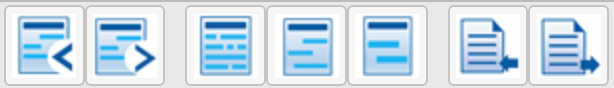
With the help of the small triangles next to the track names you can jump to the next or previous element of this track.
With the drop-down menu shown below, you can jump between different chromosomes, or specify exact positions in the Position window.

When having a track opened in the genome browser, you can drag & drop any other track over the same picture to add it to the browser, where you can find it below the bottom-most track. You can drag & drop it then to any track into the desired position.
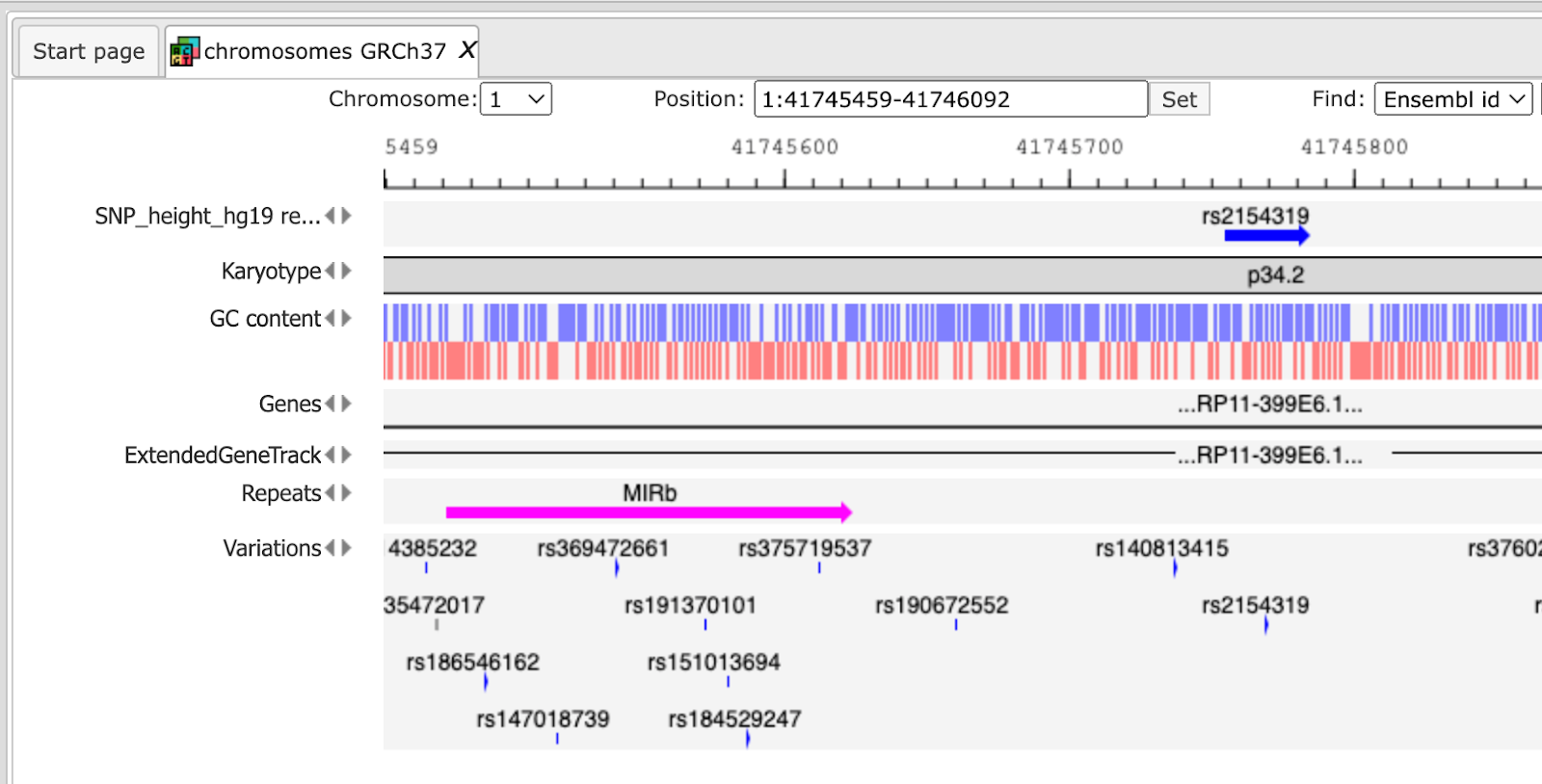
For example, you can add the track with all input SNPs from the folder All SNPs, and shift it to the top position, and then jump to the position of the 1st SNP along the chromosome. The resulting picture is shown below.
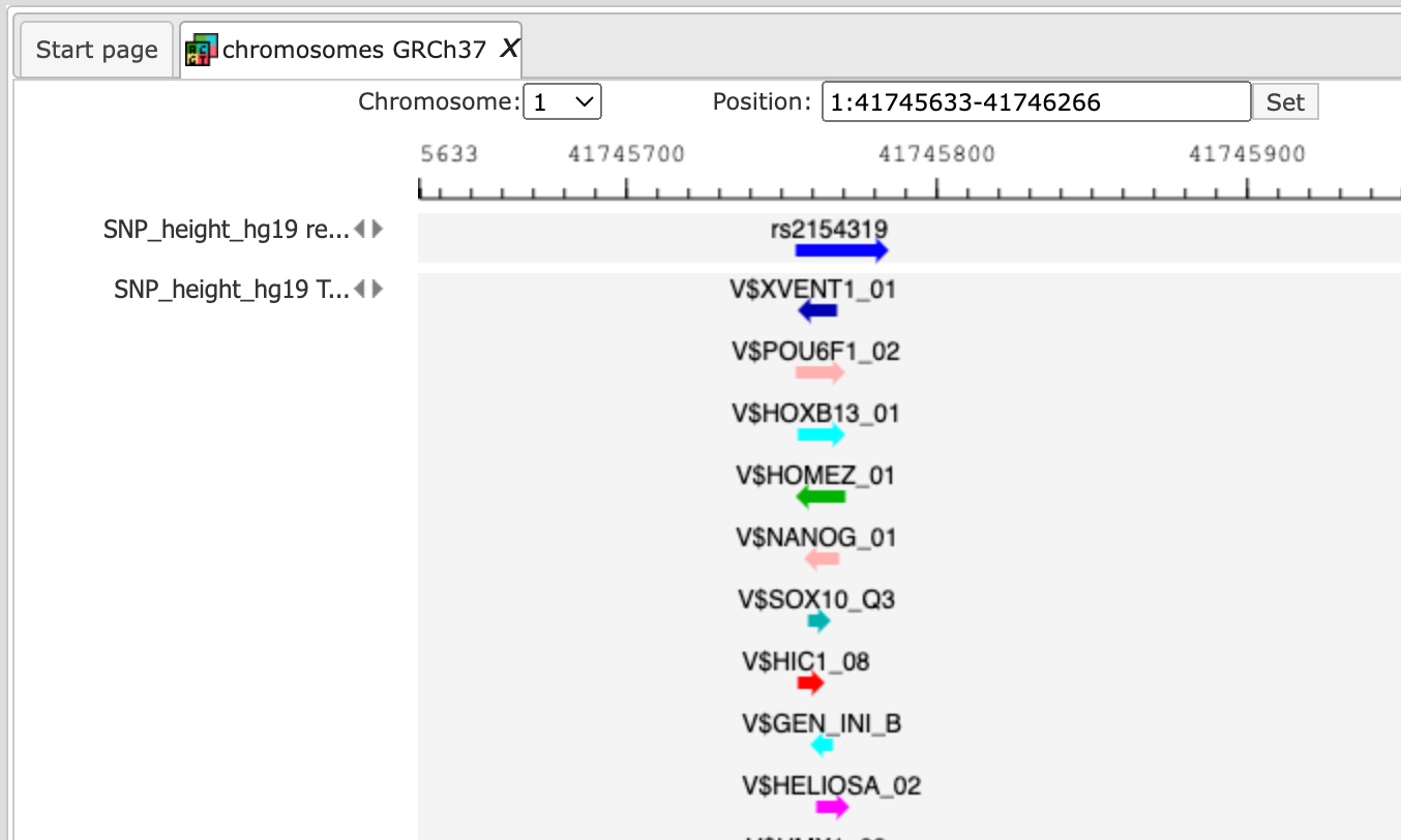
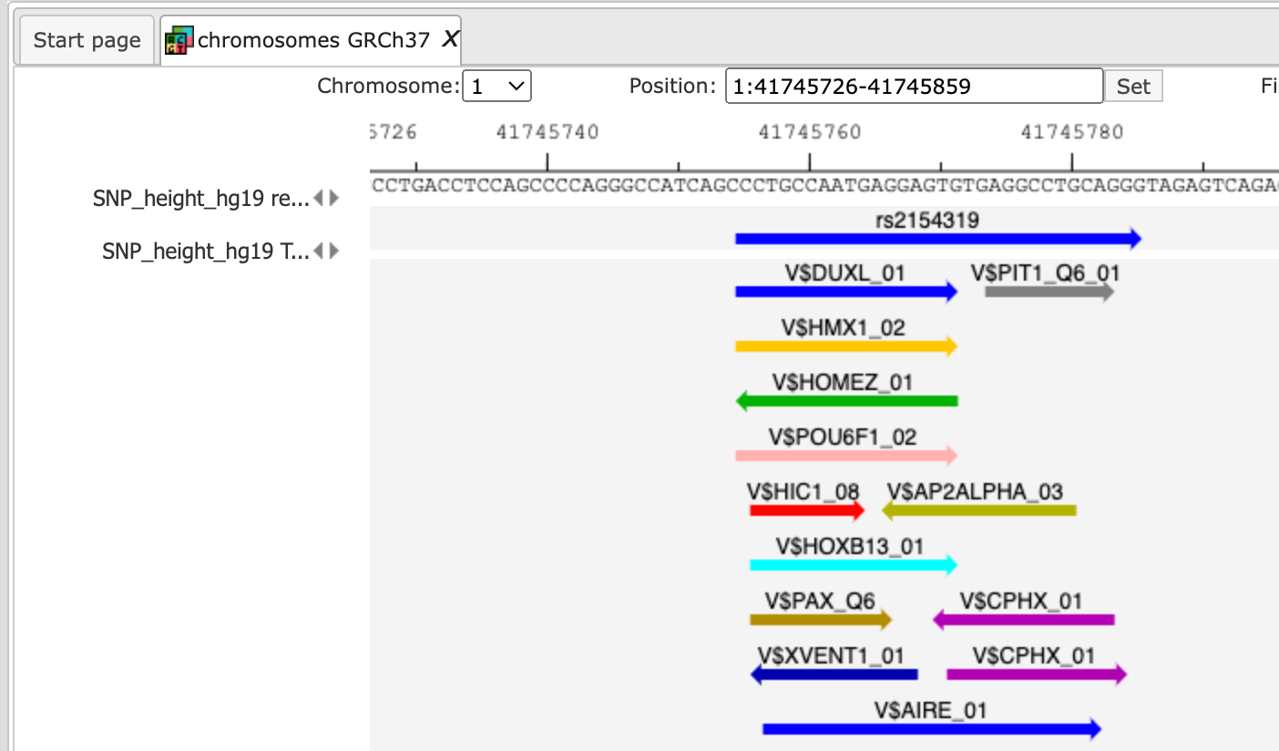
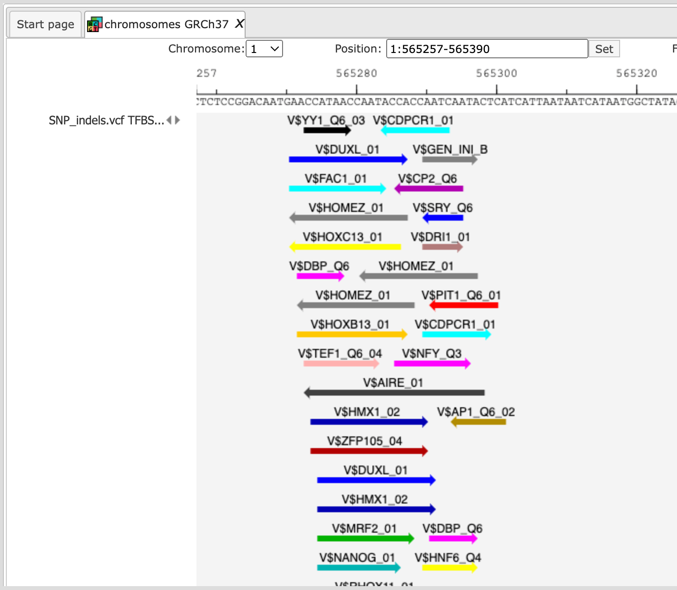
Next, you can zoom in down to the nucleotide level, and get the following picture, where one of the identified regulatory SNPs is overlapping with several TFBSs.
Note This workflow is available together with a valid TRANSFAC® license.
Please feel free to ask for details (info@genexplain.com).
Analysis with GTRD
This workflow is similar to the one described above. The difference is in the database applied for the TFBS search; in this workflow it is the GTRD database. Correspondingly, the results for regulatory SNPs overlapping with TFBSs might be different.
The results of this workflow can be found under:
Find enriched TF binding sites in variation sites
This workflow is designed to study variations (mutations) located especially within promoter regions. It helps to address the questions, which TFBSs are enriched around the variations, and which TFs are responsible for the regulation of the corresponding promoters.
As input, you submit two tracks, one track in vcf format with variations (mutations), and another track with the promoters in focus; by default all promoters from Ensembl 65.37 are used. You also need to specify a profile (a set of PWMs), and a window (region) around each variation point, e.g. 10-20 bp, where TFBS analysis is to be performed.
As output you get a summary table with enriched TFBSs, a table with transcription factors as well as a track with the enriched TFBSs, which can be used for visualization in the genome browser.
The workflow can be found on the Start page, in the section “Genomic variants”.
Step 1 Open the workflow input form from the Start page. It will open in the main Work Space and looks as shown below:
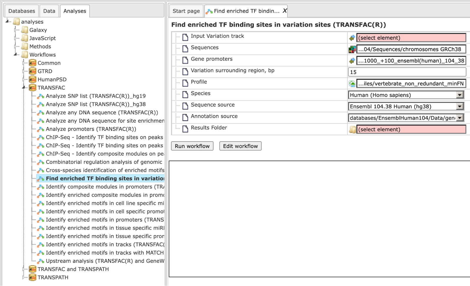
Step 2 Specify the Input Variation track in vcf format.
To specify the track, you can drag & drop it from your project within the tree
area. Alternatively, you may click on the pink field “select element” and a new
window will open, where you can select the input track. After having selected
the track, press the [Ok] button.
You can use either a newly imported track in vcf format, or a track that has been calculated within the platform, e.g. as a result of the workflow Find genome variants and indels from RNA-seq or the workflow Find genome variants and indels from full-genome NGS. Both workflows can be found under
http://platform.genexplain.com/bioumlweb/#de=analyses/Workflows/Common/
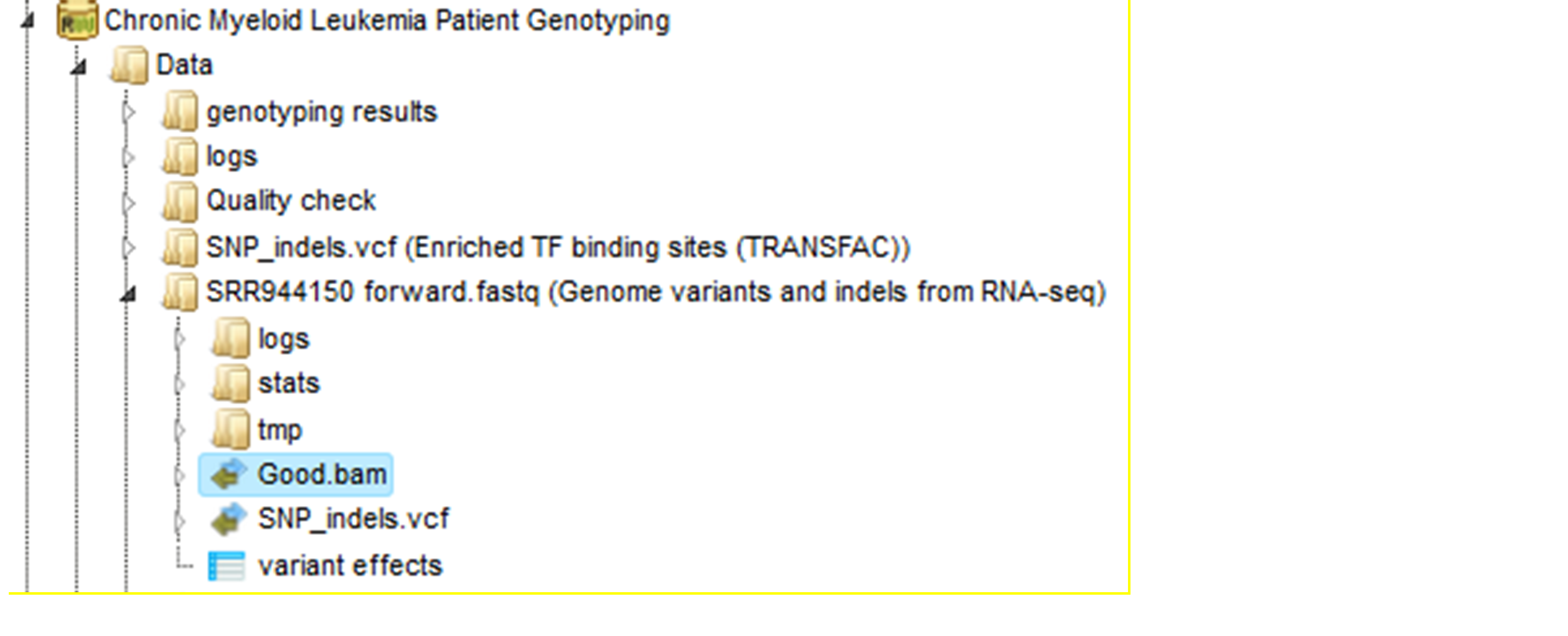
In the following example we took as input the track SNP_indels.vcf, which can be found at: https://platform.genexplain.com/bioumlweb/#de=data/Examples/Chronic%20Myeloid%20Leukemia%20Patient%20Genotyping/Data/SRR944150%20forward.fastq%20(Genome%20variants%20and%20indels%20from%20RNA-seq)/SNP_indels.vcf
This vcf file was produced by the workflow Find genome variants and indels from full-genome NGS.
Step 3 Specify the Gene promoters. By default all promoters -1000 to +100 bp relative to the TSS from Ensembl 65.37 genome version are used.
Step 4 Select the Profile. This profile will be applied for the identification of the enriched motifs around variation sites. The default profile is vertebrate_non_redundant_minSUM from the most recent TRANSFAC® release available.
Step 5 Specify the Variation surrounding region in base pairs. By default 15 bp are used. Within these region/window the search for enriched TFBSs will be performed.
Step 6 Define where the folder with the results should be located in your project tree. You can do so by clicking on the pink field “select element” in the field Results Folder, and a new window will be opened, where you can select the location of the results folder and define its name.
Start the workflow by pressing the [Run workflow] button.
Below you can see the result folder for the example:
The output folder contains one sub-folder with a track and two tables.
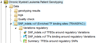
The Summary table: This table contains a list of site models (PWMs) over-represented around variation (mutation) sites in promoters, in this case 14 site models. By default this table is sorted by the Yes-No ratio, with the most over-represented model on top.
For a visualization of the over-represented TF binding sites in the variation sites you can open the SNP_indels.vcf TFBS around regulatory Variations track in the genome browser.
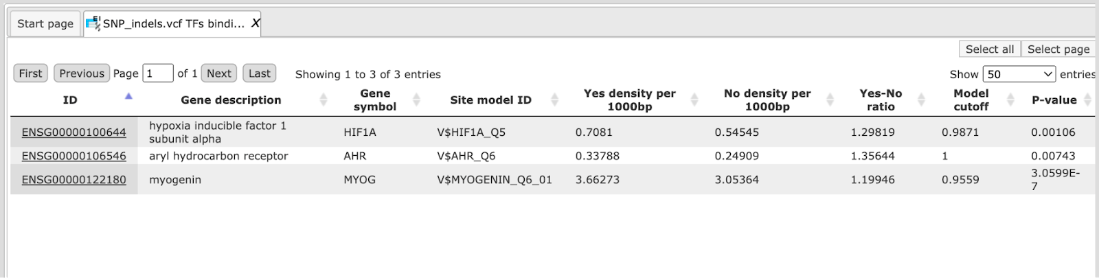
The table SNP_indels.vcf TFBS around regulatory Variations presents the list of TFs corresponding to the over-represented site models, in this case 14 TFs. This table contains the Site model IDs of over-represented binding sites, as well as the Gene description and Gene symbol for each transcription factor. The results can be sorted by Yes-No ratio, as it is shown on the screenshot below.
Mutation effect on sites analysis
This method finds transcription factor binding sites (TFBSs) affected by variations or mutations.
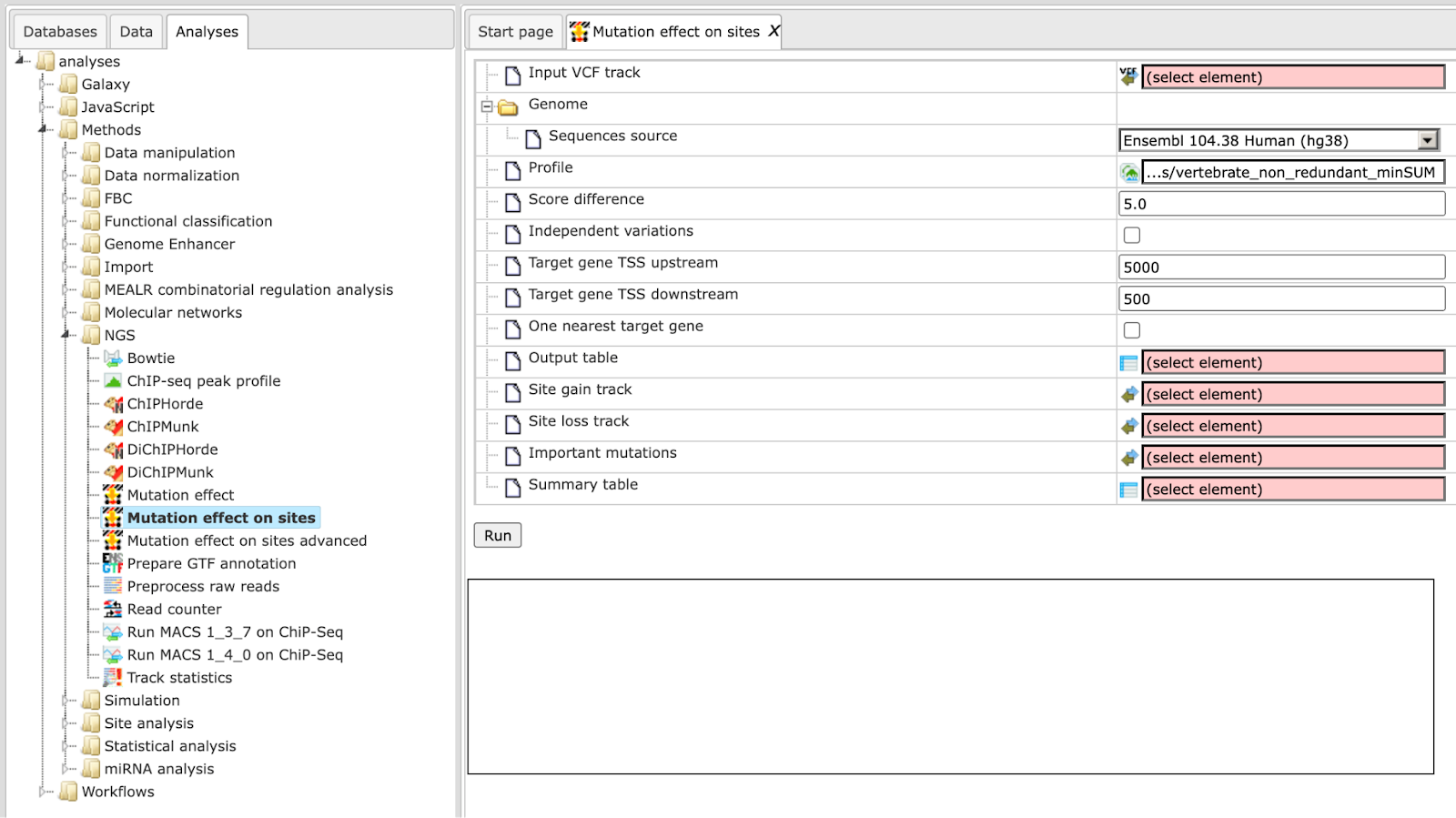
The analysis “Mutation effect on sites” can be found in the NGS folder of the analysis methods (analyses/Methods/NGS/Mutation effect on sites) or under the start page button ‘Genomic variants’ under section ‘Identify TFBS affected by genomic variations’.
Step 1 Open the analysis form from the Start page. It will open in the main Work Space and looks as shown below:
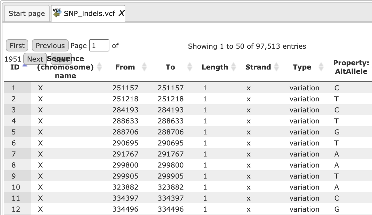
Step 2 The Input VCF track is a track file with mutations and should be in vcf format.
One input example is here on the platform:
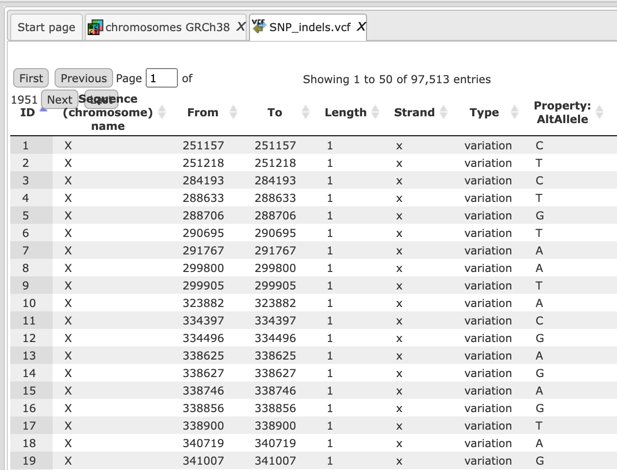
Open the track file as a table, and for each variation point you can see several columns with genomic position, chromosome, alternative nucleotide, etc., as shown below.
Step 3 Verify the Sequences source and use the drop-down menu for different Ensembl genome annotations of human, mouse and rat, as shown below.
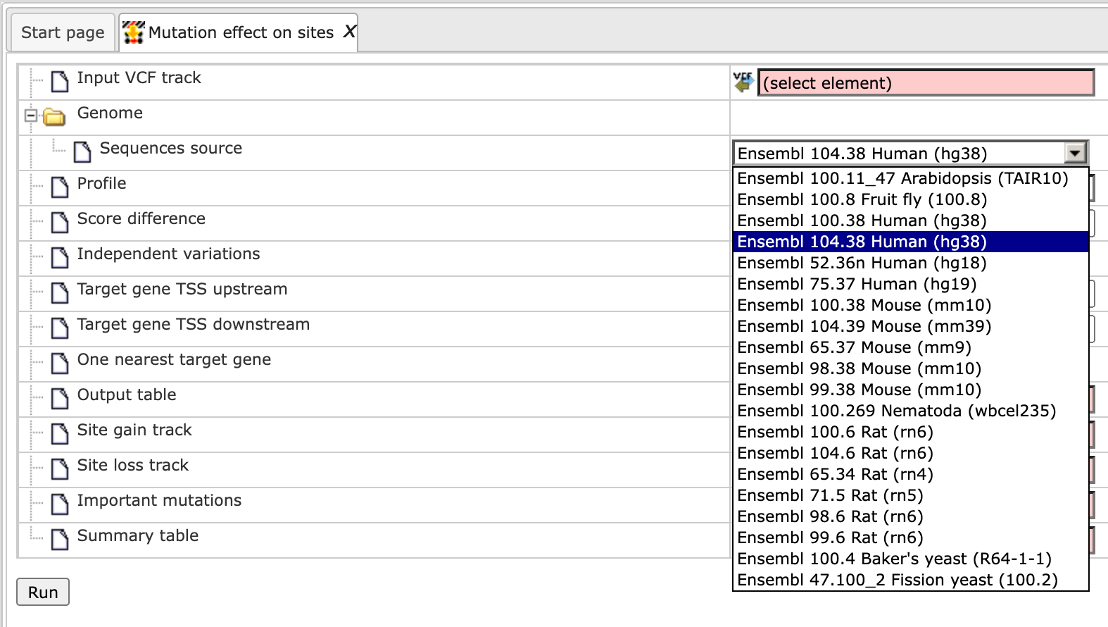
Alternatively, you can choose ‘Custom’ from the same menu, if you would like to specify another genome, e.g. a particular patient genome imported into the platform before. As soon as the option ‘Custom’ is chosen, an additional field, Sequence collection, automatically appears on the input form (screenshot below), and you can specify the sequence location manually.
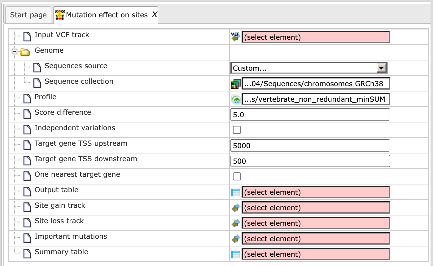
Step 4 Select the Profile. This profile will be applied for the identification of transcription factor binding sites overlapping with the variation positions. The default profile is vertebrate_non_redundant_minSUM from the most recent TRANSFAC® release available.
Step 5 The Score difference from unaffected to affected site is per default 5.0. This parameter is a threshold for the difference between the TFBS score in the reference genome and the TFBS score at the same position with a variation in the alternative sequence. For TRANSFAC matrices adjust this parameter between 0.1 and 0.5.
All TFBSs with score differences above this specified value will be reported in the output track.
The lower this value, the more TFBS will be reported as the result, because even a small change in the score will be considered. If you are interested in those TFBSs that are more strongly affected by a variation, set this parameter to 0.5 (see also example output with score difference = 0.5).
Step 6 Specify the path and name of the Output track.
After completion the output track file is found here:
is opened by default in the work space. One example of the affected identified site is shown in the red box (V$EBOX_Q6_01).
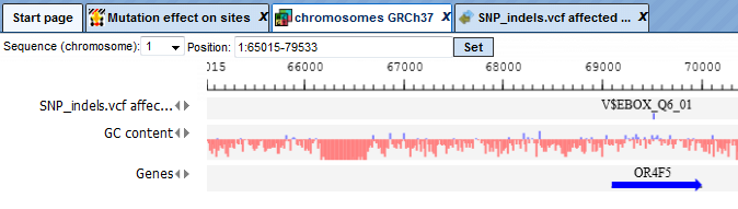
Opening the track as a table shows all affected TFBSs in table format.
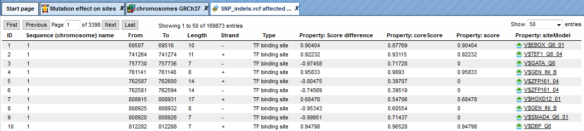
The upper example highlighted by the red box has ID=1 in the table. The columns From and To define the positions of the affected site within the genome on chromosome 1 (Sequence (chromosome) name). The column Length shows the length of the binding motif, here 10. The Type TF binding site shows that a transcription factor binding site is affected with a score difference of 0.90404.
The column Property: Score difference shows the arithmetical difference between TFBS score in the reference genome and the TFBS score at the same position with a variation (in the alternative sequence). The score difference can be positive or negative. A positive score indicates a disrupted site and a negative score predicts a new site (site appears).
A positive score difference means that the given TFBS had a better score in the reference sequence, and it was decreased by the variation. In the other words, the given variation disrupted a TFBS which occurred in the reference sequence.
A negative score means that the given TFBS has a better score in the sequence with the variation as compared to the reference sequence. A given TFBS became stronger or even appears after the variation. The conclusion can be made that a given variation created or enhanced corresponding TFBS.
The last column Property: siteModel gives a link to the matrix model and can be opened in the workspace to view the matrix logo.
SIFT (Sorting Intolerant From Tolerant) analysis
The SIFT analysis tool predicts whether a single amino acid substitution (AAS) affects protein function, based on sequence homology and the physical properties of amino acids. SIFT can be applied to naturally occurring non-synonymous single nucleotide polymorphisms (nsSNP) and laboratory-induced missense mutations. This tool uses a SQLite databases containing pre-computed SIFT scores and annotations for all possible nucleotide substitutions at each position in the human exome. Allele frequency data are from the HapMap frequency database, and additional transcript and gene-level data are from Ensembl BioMart. The updated version of SIFT is published in Nat Protoc. 4:1073-1081, 2009.
The tool can be found in the Galaxy section of the geneXplain platform (analyses/Galaxy/Human Genome Variation/SIFT) or on the start page button ‘Genomic variants’ under section ‘Identify TFBS affected by genomic variations’.
Step 1 Open the analysis form from the Start page. It will open in the main Work Space and looks as shown below:
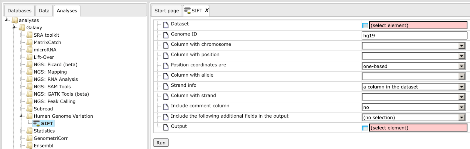
Step 2 The input Dataset must contain columns for the chromosome, position, and alleles. The alleles must be two nucleotides separated by ‘/’, usually the reference allele and the allele of interest. The strand must either be in another column.
Input example format:
chr3 81780820 + T/C \
chr2 230341630 + G/A \
chr2 43881517 + A/T
chr2 43857514 + T/C
chr6 88375602 + G/A
chr22 29307353 - T/A \
chr10 115912482 - G/T\
chr10 115900918 - C/T\
chr16 69875502 + G/T \
One example input table can be found here on the platform:
Step 3 Determine the Genome ID. The tool currently works only for genome builds hg18 or hg19.
Step 4 Define the Column with chromosome. In our example above it is column 5 (SNP_matching-Chromosome).
Step 5 Define the Column with position. In our example above it is column 6 (SNP_matching-Position).
Step 6 Selection if Position coordinates are one-based (default) or zero-based counted.
Step 7 Define the Column with allele. In our example above it is column 7 (SNP_matching-Allele).
Step 8 Define whether the Strand info is a column in the dataset (default).
Step 9 Define the Column with strand. In our example above it is column 8 (SNP_matching-Strand).
Step 10 Select Include comment column for additional comments.
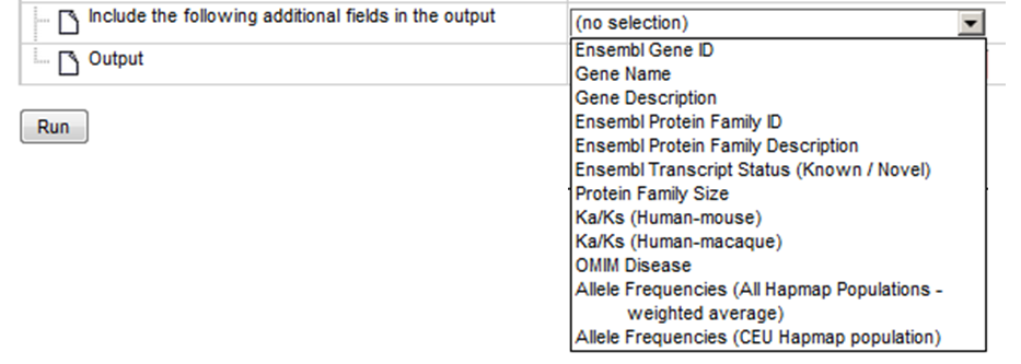
Step 11 Possibility to select multiple output columns and Include the following additional fields in the output table.
Step 12 Define where the output table should be located in your project tree. You can do so by clicking on the pink field “select element” in the field Output, and a new window will be opened, where you can select the location of the table and define its name.
Start the SIFT analysis by pressing the [Run workflow] button.
An example output table can be found here:
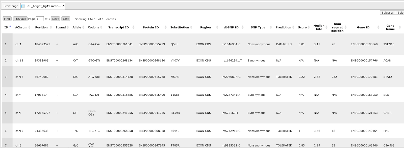
The column Codons in the output table shows the originally and changed codon of the input position coordinates. The Transcript ID and Protein ID give information about the affected gene/protein. If the SNP Type is Nonsynonymous, the Prediction of the protein function is DAMAGING, which means that the functionality of the protein is predicted as being compromised.
Selected additional fields like Gene ID, Gene Name and others are shown in the output table.