RNA-seq
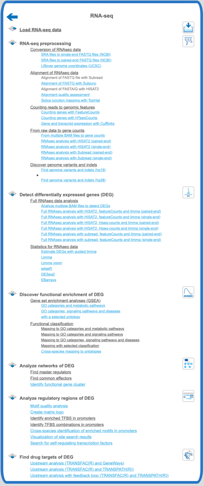
When you click on the tiled button “RNA-seq” in the Work Space of the on the start page, the following listing will appear:
RNA-seq preprocessing
SRA to FASTQ
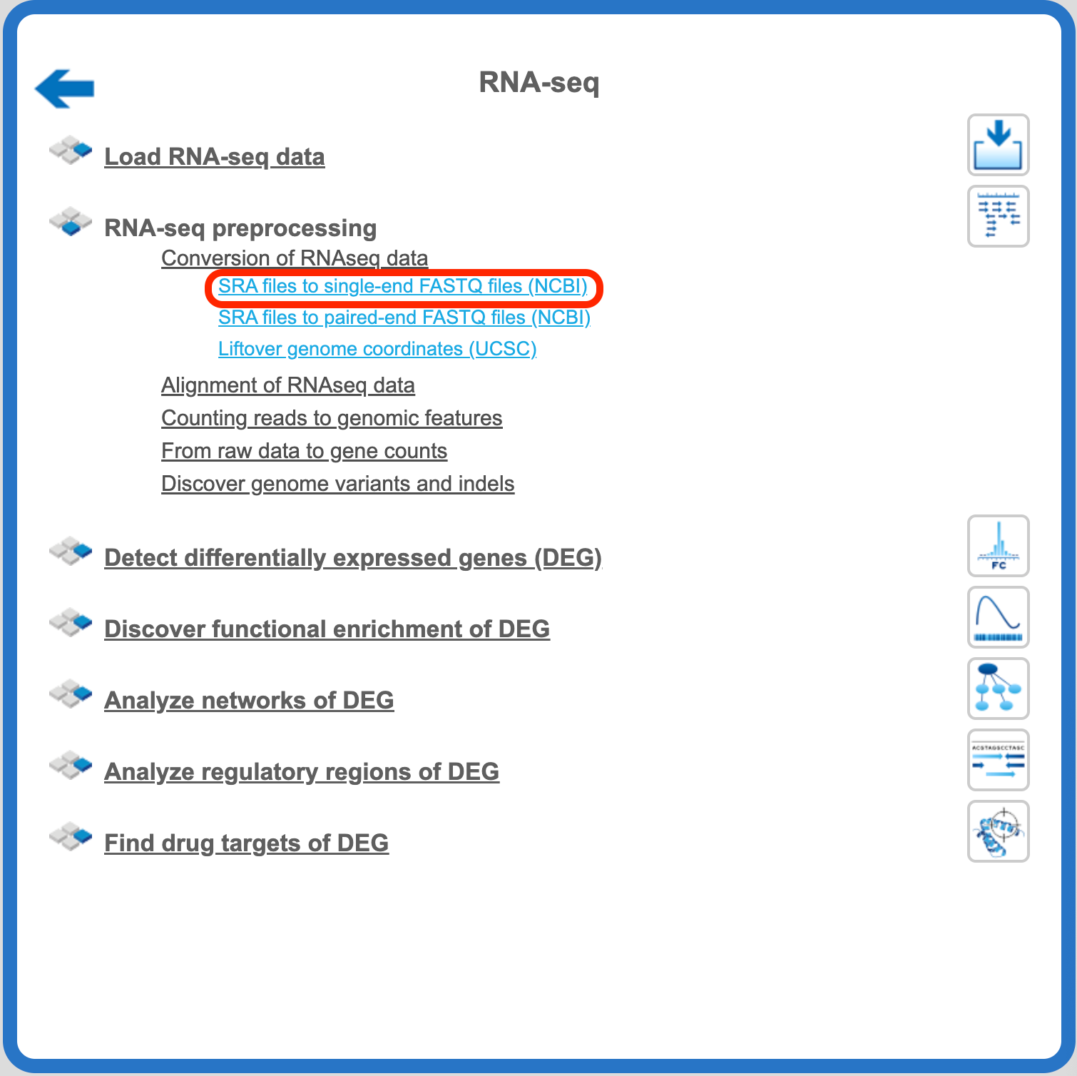
This workflow can be used to convert SRA data files (e. g. from NGS/RNA-seq experiments) into FASTQ files. The FASTQ format is widely used by a number of tools and the geneXplain platform is among them; on the other hand, NGS data are often collected in SRA format, thus the conversion of SRA format into FASTQ format is an important function. An example of public data stored in SRA format can be found here (https://www.ncbi.nlm.nih.gov/sra?term=SRP051443) and can be uploaded directly via FTP import into the geneXplain platform. The workflow “SRA to FASTQ” can be found on the Start page, under the NGS/RNA-seq button.
To launch the workflow, follow these steps:
Step1. Open the workflow input form from the Start page. It looks as shown below:
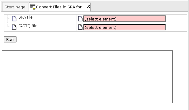
Step 2. Specify the folder with the SRA files in the field Input folder. You can drag it from your project within the tree area and drop it in the box beside the folder pictogram. Alternatively, you may click on the field (select element) and a new window will be opened, where you can select the input folder.
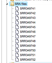
It contains 12 files in SRA format as shown below. Please note, this folder occupies 1.5 GB work space.
The output folder name and folder path is automatically created, but can be changed in a user-specific way.
Press [Run workflow] and wait till the workflow is completed.
Example of an output folder:
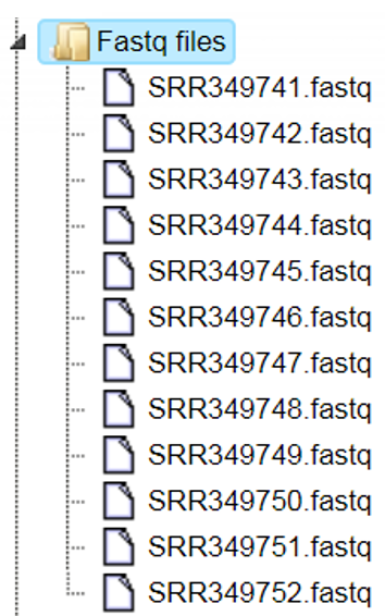
The output folder contains 12 files with the same names and now with the extension fastq. Please note, the size of the output folder is 16.6 GB.
Note Working with NGS data in SRA and FASTQ formats requires substantial work space available in your user account. Feel free to contact us (info@genexplain.com) to upgrade your account with additional disk space.
Convert genome coordinates with Lift-Over
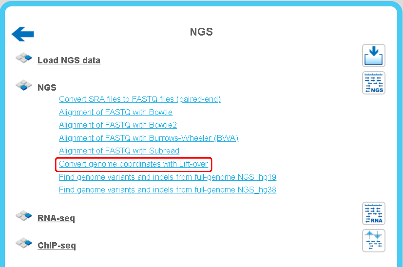
While working with NGS data, quite often it might quite often be required to convert positions from one genome assembly to another one, and The Lift-Over program can be applied for this task. Within the geneXplain platform, you can find it on the Start page under the NGS button, as highlighted below.
This tool is based on the LiftOver utility and Chain track from the UC Santa Cruz Genome Browser.
It converts coordinates and annotations between assemblies and genomes. The input is a track with genomic positions according to a particular genome assembly, and the output is a track with positions according to another genome assembly.
To launch the workflow, follow these steps:
Step1. Open the input form from the Start page. It looks as shown below:
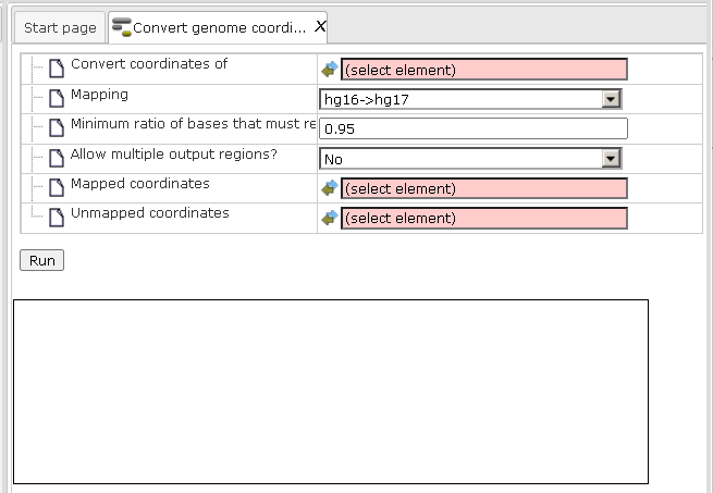
Step 2. Specify the input track in the field Convert coordinates of. You can drag it from your project within the tree area and drop it in the box of the field.
The further steps of the workflow are demonstrated by means of the tables in one of the pre-prepared examples. You can find these tables here:
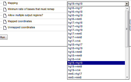
Step 3. Specify the Mapping of the input track by selecting the desired genome conversion from the drop-down menu.
In the majority of cases not everything can be remapped to another assembly. The minimum ratio of bases that must be re-mapped is by default 0.95, you can change this by typing in this field.
Step 4. Allow multiple output regions: choose Yes or No.
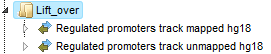
Step 5. Define where the output tracks should be located in the tree. The method produces two output tracks, one containing all the mapped coordinates and the other containing the unmapped coordinates (if existing).
After filling out all input fields press [Run] and wait till the method is completed.
The output is a folder with two tracks as shown below:
Alignment of FASTQ with Bowtie
Bowtie is a short-read aligner designed to be ultrafast and memory-efficient. It was developed by Ben Langmead and Cole Trapnell (Langmead B, Trapnell C, Pop M, Salzberg SL. Ultrafast and memory-efficient alignment of short DNA sequences to the human genome. Genome Biology 10:R25). The Bowtie method can be found in the Galaxy section of the platform (analyses/Galaxy/solexa_tools/bowtie_wrapper).
Input format: Bowtie accepts files in Sanger FASTQ format. Often, the sequence files are represented in SRA format (Sequence Read Archives). This format is used to deposit sequences at the Sequence Read Archives at NCBI, EBI, and DDBJ. Please consider converting the SRA files into FASTQ files before starting Bowtie. You can use the conversion tool Convert Files in SRA format to FASTQ or Convert Files in SRA format to paired FASTQ in the Galaxy section of the platform (analyses/Galaxy/sra_toolkit/fastq-dump).
To launch the Bowtie tool, follow these steps:
Step1. Open the Bowtie input form from the Start page by clicking on Alignment of FASTQ with Bowtie option in the RNA-seq preprocessing subsection. It will open in the main Work Space and looks as shown below:
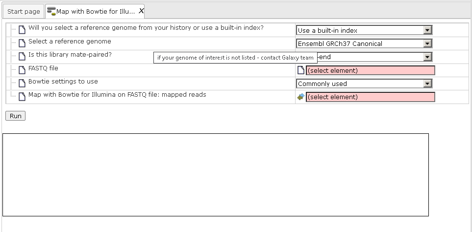
Step 2. Specify the reference genome.
The field Will you select a reference genome from your history or use a built-in index? defines the reference genome. If you keep the default “Use a built-in index” the program makes an alignment to the reference genome which is provided as part of the platform (the genome builds for human, mouse and rat are provided). Depending on the species used, please specify hg19 for human, mm9 for mouse and rn4 for rat in the next field Select a reference genome.
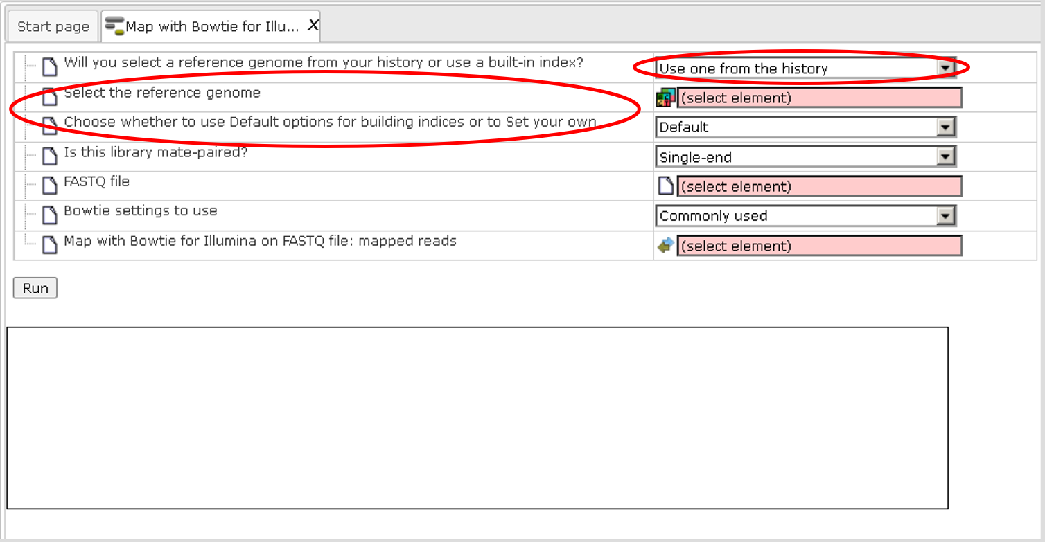
If you select the “Use one from the history” option in the 1st field, two new fields will appear in the form: Select the reference genome and Choose whether to use Default options for building indices or to Set your own, as shown in the screenshot below, highlighted by the red ovals. In this case you should provide a preloaded reference genome (preloaded in Fasta, EMBL or GeneBank formats) and choose how to build sequence indices which will be used by the alignment algorithm of Bowtie.
Step 3. The field Is this library mate-paired? defines the type of the sequence library which was used in NGS sequencing. The default is Single-end, the alternative is Paired-end. You should know this detail about your library of short reads.
Step 4. Specify the input file in the field FASTQ file. You can either drag-and-drop or select the file name from the Tree area. Here, as an example, we use data from a published RNA-seq experiment analyzing the human esophageal squamous cell carcinoma (ESCC), GSE32424. FASTQ files are found here: https://platform.genexplain.com/bioumlweb/#de=data/Examples/RNA-Seq%20analysis%20of%20human%20esophageal%20squamous%20cell%20carcinoma%20(ESCC),%20GSE32424,%20FASTQ%20files/Data/Fastq%20files
This example contains results of an RNA-seq Illumina NGS sequencing of twelve clinical samples from human esophageal squamous cell carcinoma (ESCC) (seven tumors and five non-tumors). The authors provided sequences as so-called non-aligned BAM files. We loaded these BAM files directly from GEO as one archive using the ftp uploading function of the geneXplain platform. After that, we converted the non-aligned BAM files into FASTQ files using the tool: SAM to FASTQ from the NGS: Picard (beta) subsection of the Galaxy section of the platform (analyses/Galaxy/picard_beta/picard_SamToFastq).
Step 5. The field Bowtie settings to use is set by default to Commonly used. If you change it to the Full parameter list from the drop-down menu, a full list of parameters of the alignment algorithm is enabled for editing. The full description of all these parameters is given in the original paper of Langmead et al. mentioned above which describes the algorithm of Bowtie.
Step 6. Please keep the box Suppress the header in the output SAM file unchecked (as it is by default) to generate SAM/BAM output files suitable for further use by Cufflinks tool.
Step 7. Set the output file name (for the output BAM file) in the field Map with Bowtie for Illumina… and press the button [Run].
Tip It is recommended to save the output file into a separate folder containing all BAM output files from one particular experiment. This will allow you to run the next workflow for the quantification of all SAM/BAM files from this defined folder.
Results
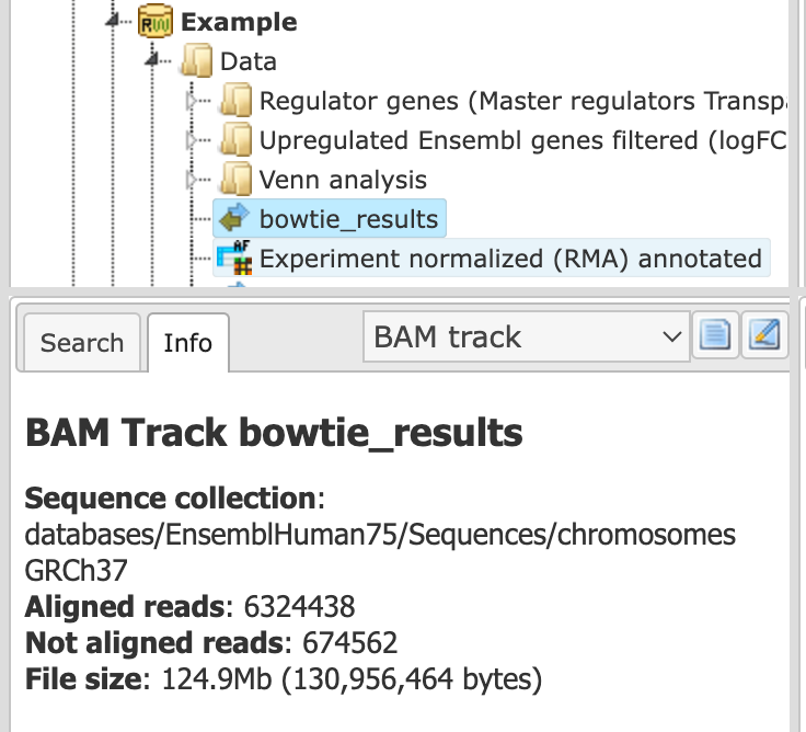
The result of this method is one BAM file which is generated by the Bowtie program as the result of the alignment of the sequence reads from the input FASTQ file to the reference genome.
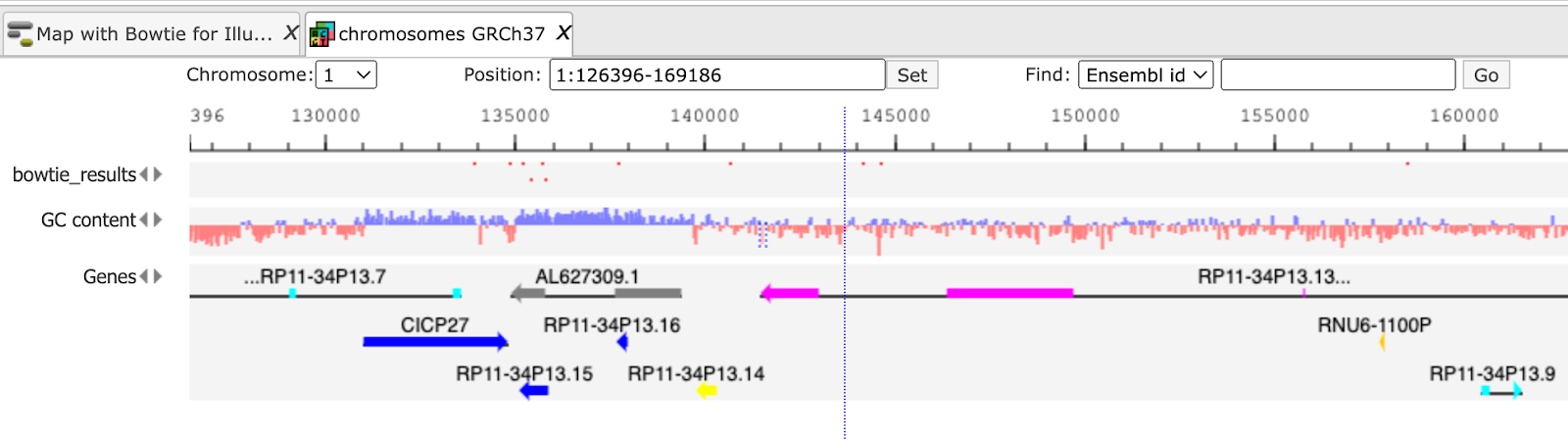
Generated BAM file is a track and has the ( ) icon in the tree. As usual for all tracks, it opens in the Work Space. You can see the positions of each aligned read in the genome and upon zooming-in you get all detailed information about each read complete with sequence, length, and quality.
In the info box you can see information about the output BAM file. The number of aligned and not aligned reads and overall file size is shown.
Note The input FASTQ and output BAM files of the Bowtie tool require a considerable amount of working space. One FASTQ file can occupy several GB of space. If you need more space for storage and work with your FASTQ and BAM files, please feel free to ask for details (info@genexplain.com).
Find genome variations and indels from RNA-seq
The challenge of obtaining accurate variant calls from RNA-seq data is substantial. The workflow is based on a framework to discover genotype variations published by De Pristo et al., Nature Genetics 43:491-498, 2011. The process applied includes initial read mapping, local realignment around indels, base quality score recalibration, SNP discovery and genotyping to find all potential variants.
The workflow can be found in the section “RNA-seq Preprocessing”.
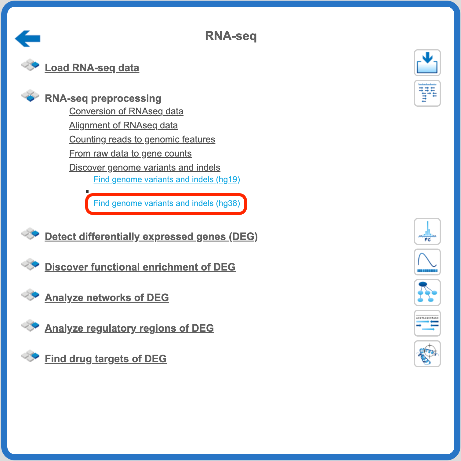
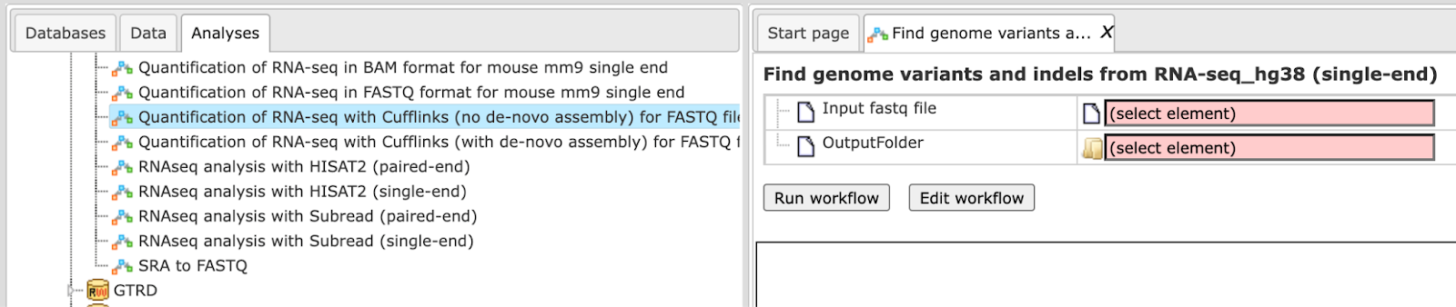
Step 1. Open the workflow input form from the Start page. It will open in the main Work Space and looks as shown below:
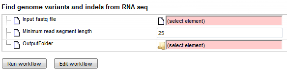
Step 2. Specify the input file in FASTQ format in the field Input fastq
file.
To specify the fastq file, you can drag & drop it from your project within the
tree area. Alternatively, you may click on the pink field “select element” and a
new window will open, where you select the input track. After having selected
the track, press the [Ok] button.
Step 3. Specify the Minimum read segment length. By default a minimum length of 25 is given.
Step 4. Define where the folder with the results should be located in your project tree. You can do so by clicking on the pink field “select element” in the field OutputFolder, and a new window will be opened, where you can select the location of the results folder and define its name.
Start the workflow by pressing the [Run workflow] button.
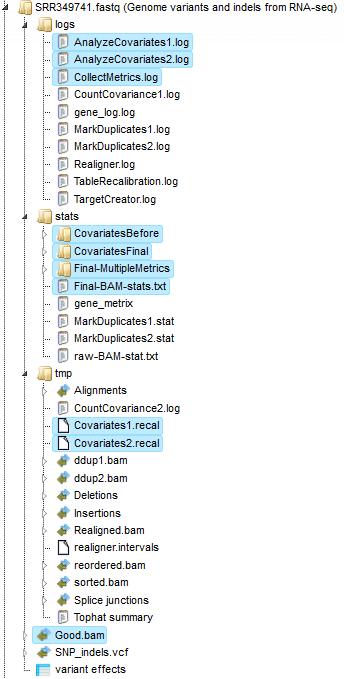
In the following example we took as input the fastq file [SRR349741.fastq]
The output folder can be found here: https://ge.genexplain.com/bioumlweb/#de=data/Examples/RNA-Seq%20analysis%20of%20human%20esophageal%20squamous%20cell%20carcinoma%20(ESCC)%2C%20GSE32424%2C%20FASTQ%20files/Data/SRR349741.fastq%20(Genome%20variants%20and%20indels%20from%20RNA-seq)/summary_hisat2
The output folder contains several files and subfolders with all results of the analysis.
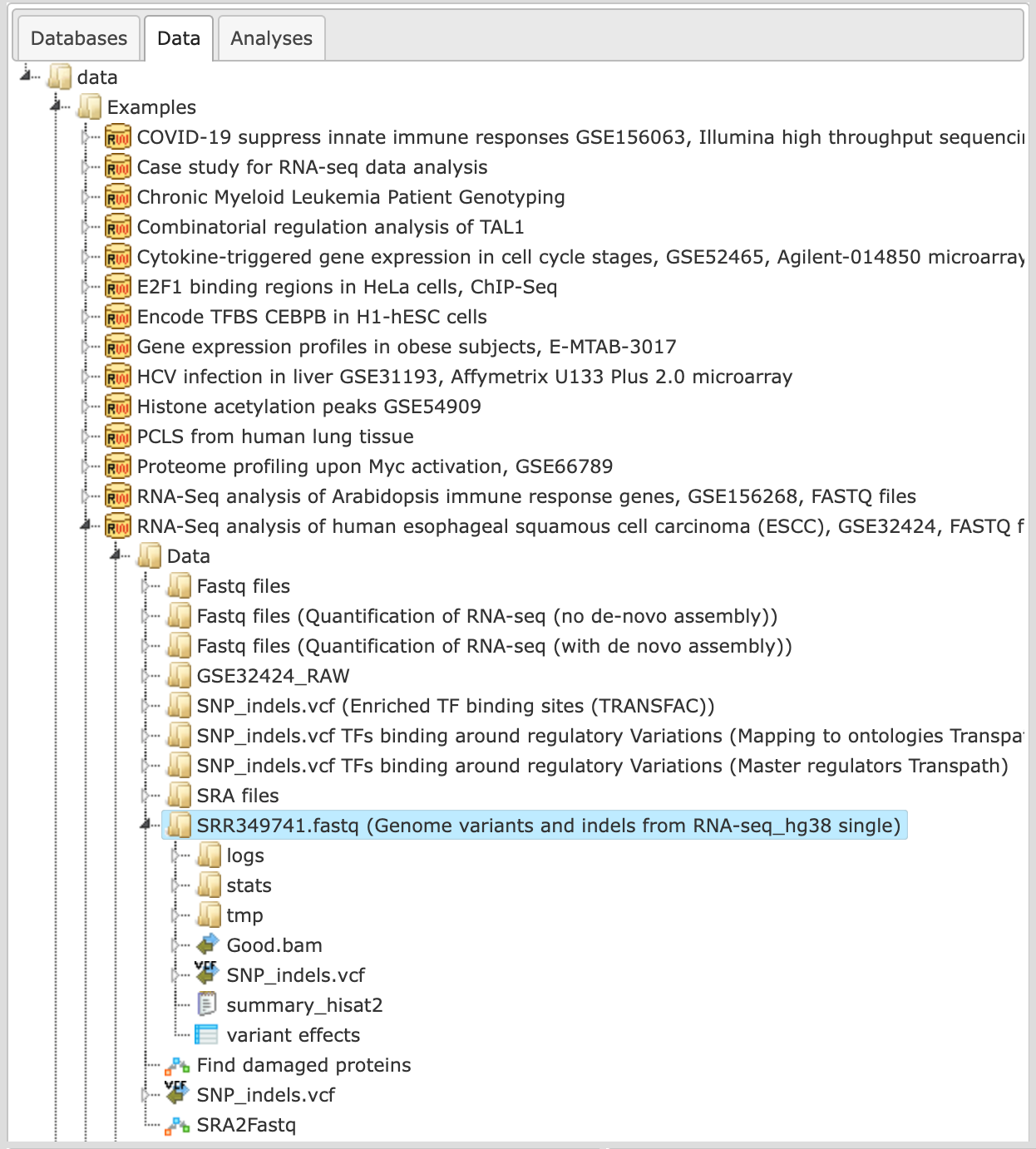
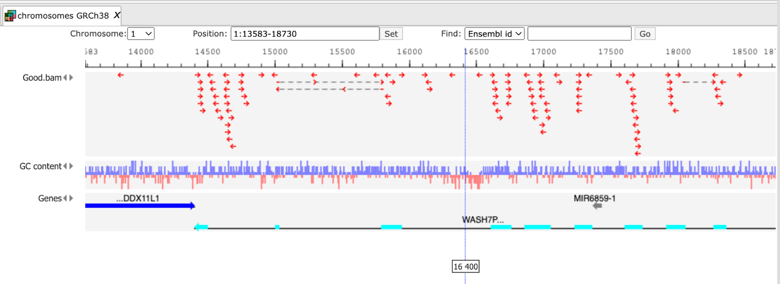
The first step of the workflow is an alignment of all reads of fastq file using the HISAT2 tool. In the result folder one can see a sub-folder “tmp” which contains all found indels. They are stored as tracks and can be opened in the genome browser by double-click on each of the tracks. Each short line (arrow in the higher zoom) represents an aligned “read” from the fastq file.
The initial alignments are sorted and reordered to prepare the next quality checking steps. The results of these two steps are stored in the folder tmp as the two files reorder.bam and sorted.bam.
The next step removes duplicates. The purpose is to mitigate the effects of PCR amplification bias introduced during library construction. Two read pairs are considered duplicate if they align to the same genomic position. The resulting MarkDuplikates1.log file is stored in the log folder and the MarkDuplikates1.stat file is stored in the stat folder.
The next step is a local realignment. Read mapping algorithms operate on each read independently, locally realign reads such that the number of mismatching bases is minimized across all the reads. Output files are Realigner.log and TargetCreator.log in the log folder, ddup1.bam, Realigned.bam and realigner.intervals in the tmp folder.
The realigned BAM file is used again to remove duplicates (output MarkDuplicates2.log and MarkDuplicates2.stat), because realignment may change genomic positions of read pairs. After this step additional duplicates can be identified. The next step is a recalibration of base quality values. For each base in each read various covariates (such as reported quality score, position in read, dinucleotide, read GC-content) are calculated. Using these values the algorithm builds the model that predicts sequencing errors. Then it applies this model to calculate an empirical base quality score and overwrites the phred quality score currently in the read. Output is a new BAM file (Good.bam).
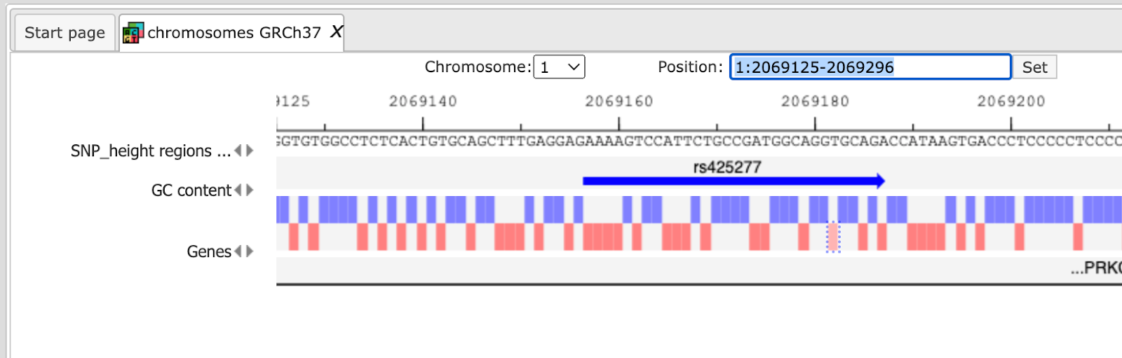
This file is used for the unified GATK which is the next step of this workflow (Genome Analysis Toolkit) genotyper method to detect the SNP-indels (table in VCF format) which the user can visualize by double click.
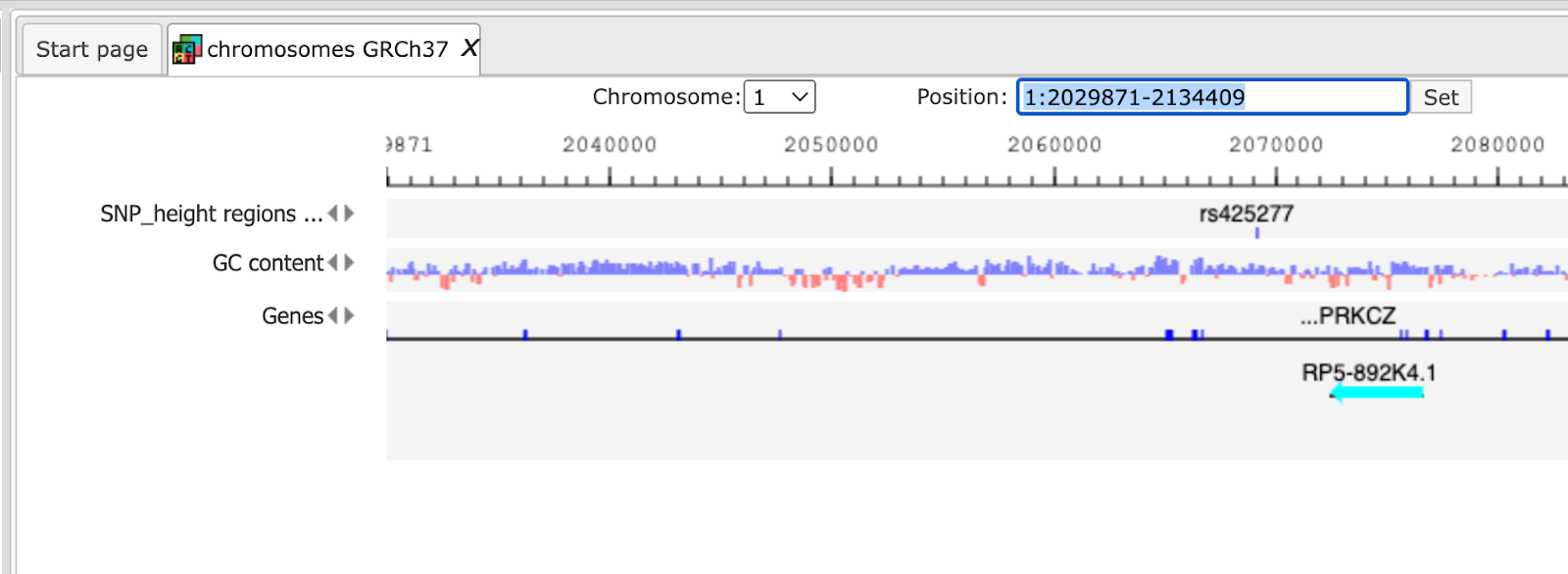
After Zooming in information of variation on nucleotide basis is shown.
In the next step each identified variation (SNP_indels) is analysed with the help of the “variant_effect_predictor” algorithm
https://platform.genexplain.com/bioumlweb/#de=analyses/Galaxy/ensembl/variant_effect_predictor
As a result it creates a final table that gives detailed information about each variation as shown in the example below:
Quantification of RNA-seq with Cufflinks (no de-novo assembly) for FASTQ files
This workflow offers a possibility to discover new genes and transcripts (splice variants) and measure transcript expression in a single assay from RNA-seq data. This workflow is described in “Differential gene and transcript expression analysis of RNA-seq experiments with TopHat and Cufflinks”, Nat. Protoc. 7:562-578, 2012.
Step 1. Open the workflow input form from the Start page. It will open in the main Work Space and looks as shown below:
Step 2. Specify the Experiment fastq files and the Control fastq
files.
To specify the input files in Sanger FASTQ format, you can drag & drop it from
your project within the tree area.
Step 3. Define where the folder with the results should be located in your project tree. You can do so by clicking on the pink field “select element” in the field Output folder, and a new window will be opened, where you can select the location of the results folder and define its name.
Start the workflow by pressing the [Run workflow] button.
Results can be accessed here:
Read alignment with TopHat
The first step of the workflow is alignment of sequence reads with TopHat (http://tophat.cbcb.umd.edu/). TopHat aligns reads to the genome and discovers transcript splice sites. TopHat uses Bowtie (http://bowtie-bio.sourceforge.net/index.shtml) as an alignment ‘engine’ and breaks up reads that Bowtie cannot align on its own into smaller pieces called segments.
Output files are tables and tracks with insertions, deletions, splice junctions and the alignments.
Example output is opened as track:
Mismatches, insertions and deletions in the alignments can identify polymorphisms between the sequenced sample and the reference genome, or even pinpoint gene fusion events in tumor samples. Reads that align outside annotated genes are often strong evidence of new protein-coding genes and noncoding RNAs. RNA-seq read alignments can reveal new alternative splicing events and isoforms. Alignments can also be used to accurately quantify gene and transcript expression, because the number of reads produced by a transcript is proportional to its abundance.
Differential analysis with Cuffdiff
The second step of the workflow is performed by Cuffdiff, part of the Cufflinks package, which calculates expression in two or more samples and tests the statistical significance of each observed change in expression between them. Cuffdiff allows for supplying multiple technical or biological replicate sequencing libraries per condition. With multiple replicates, Cuffdiff learns how read counts vary for each gene across the replicates and uses these variance estimates to calculate the significance of observed changes in expression.
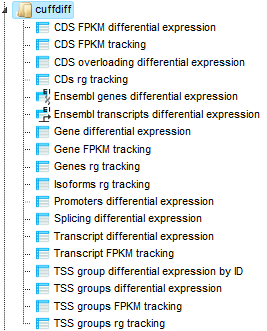
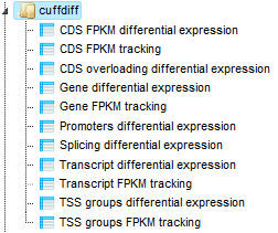
Cuffdiff reports 15 output files:
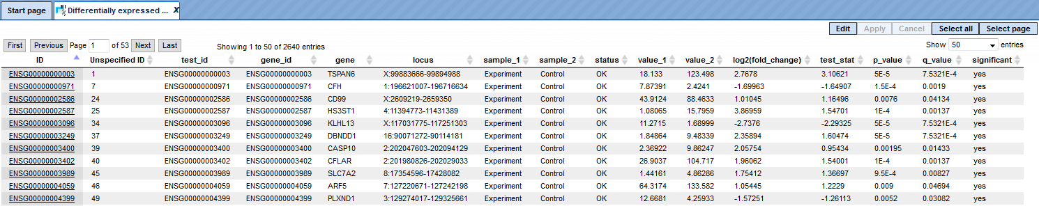
The last step of the workflow comprises several conversions and filtering steps of some Cuffdiff output files. The final table and tracks are in the result folder:
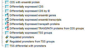
The table Differentially expressed Ensembl genes contains all identified differentially expressed genes (Ensembl IDs) (also converted into a table of transcripts and a table of TRANSPATH® proteins).
The Regulated promoters are extracted from the table Differentially expressed Ensembl transcripts. Transcripts with the same transcription start site (TSS) are merged into the single ‘TSS group’ and Differentially expressed TSS groups are also identified. Regulated promoters from TSS groups are identified using those TSS groups. Similarly, Differentially expressed CDS groups are identified (CDS group is the group of transcripts with the same coding sequence; they produce exactly the same protein). And CDS group table is used to find Differentially expressed TRANSPATH proteins from CDS groups.
Quantification of RNA-seq with Cufflinks (with de-novo assembly) for FASTQ files
This workflow offers the ability to discover new genes and transcripts (splice variants) and measure transcript expression in a single assay from RNA-seq data. This workflow is described in “Differential gene and transcript expression analysis of RNA-seq experiments with TopHat and Cufflinks”, Nat. Protoc. 7:562-578, 2012.
Step 1. Open the workflow input form from the Start page. It will open in the main Work Space and looks as shown below:
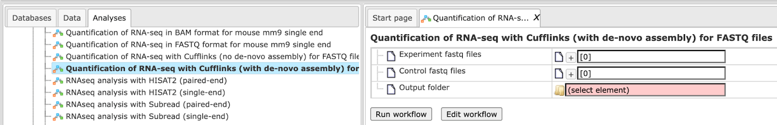
Step 2. Specify the Experiment fastq files and the Control fastq
files.
To specify the input files in Sanger FASTQ format, you can drag & drop it from
your project within the tree area.
Step 3. Specify the Reference annotation.
Step 4. Specify the Reference sequence.
Step 5. Define where the folder with the results should be located in your project tree. You can do so by clicking on the pink field “select element” in the field Output folder, and a new window will be opened, where you can select the location of the results folder and define its name.
Start the workflow by pressing the [Run workflow] button.
Read alignment with TopHat
The first step of the workflow is a read alignment with TopHat (http://tophat.cbcb.umd.edu/). TopHat aligns reads to the genome and discovers transcript splice sites. TopHat uses Bowtie (http://bowtie-bio.sourceforge.net/index.shtml) as an alignment ‘engine’ and breaks up reads that Bowtie cannot align on its own into smaller pieces called segments.
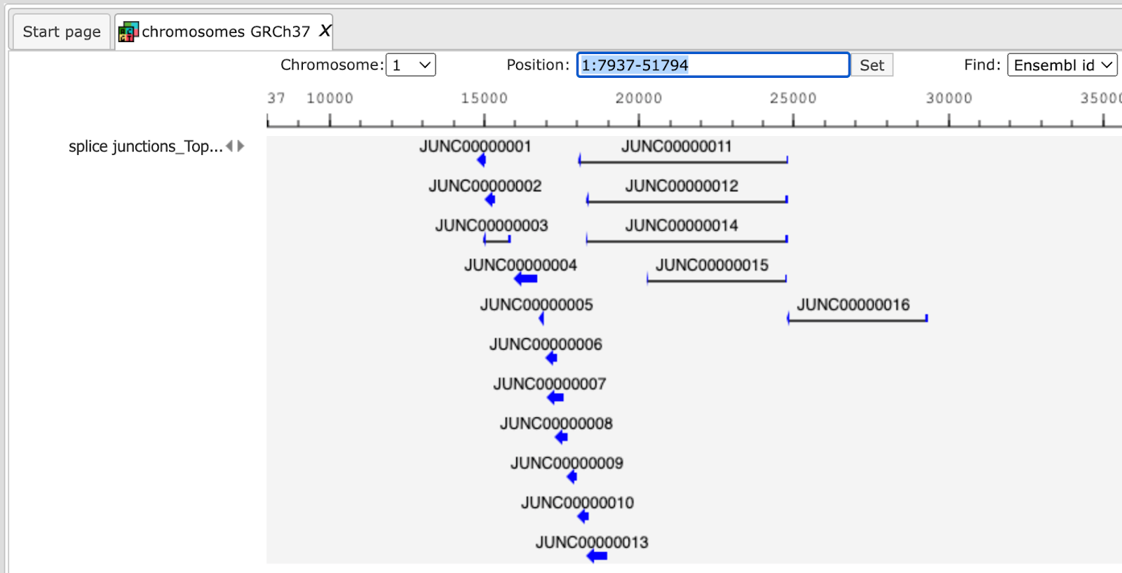
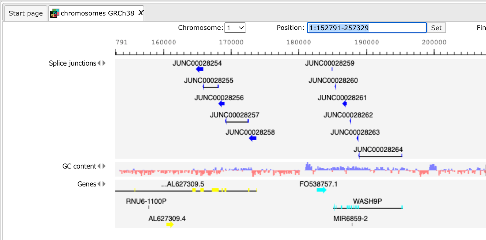
Output files are tables and tracks with insertions, deletions, splice junctions and the alignments.
Example output of splice junctions
opened as track is shown below:
Mismatches, insertions and deletions in the alignments can identify polymorphisms between the sequenced sample and the reference genome, or even pinpoint gene fusion events in tumor samples. Reads that align outside annotated genes are often strong evidence of new protein-coding genes and noncoding RNAs. RNA-seq read alignments can reveal new alternative splicing events and isoforms. Alignments can also be used to accurately quantify gene and transcript expression, because the number of reads produced by a transcript is proportional to its abundance.
Transcript assembly with Cufflinks
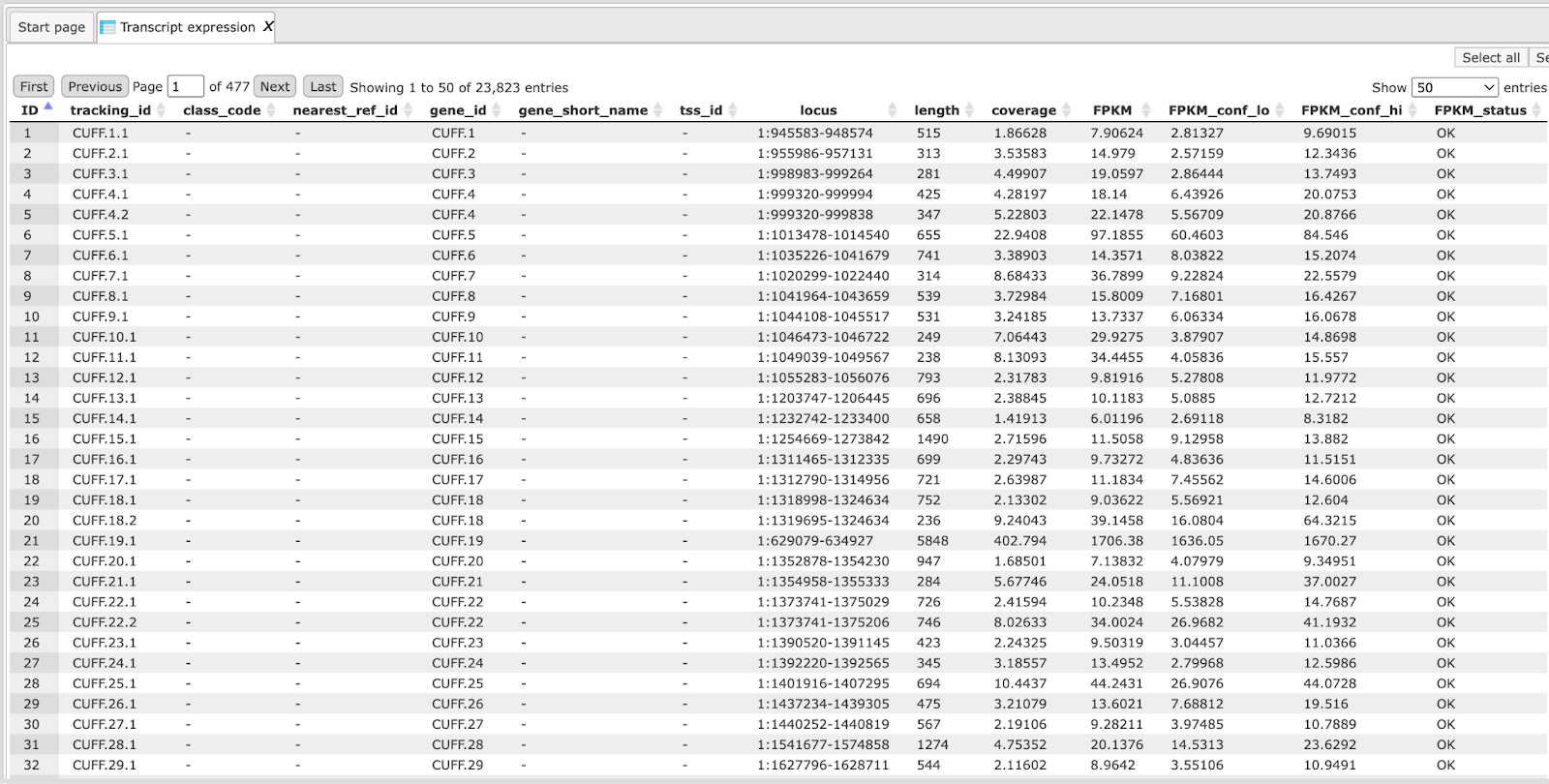
Cufflinks uses the alignments to map reads against the genome and to assemble the reads into transcripts. Cufflinks assembles individual transcripts from RNA-seq reads that have been aligned to the genome. Because a sample may contain reads from multiple splice variants for a given gene, Cufflinks must be able to infer the splicing structure of each gene. Thus, Cufflinks reports a parsimonious transcriptome assembly of the data. The algorithm reports as few full-length transcript fragments or ‘transfrags’ as are needed to ‘explain’ all the splicing event outcomes in the input data. Output tracks of Cufflinks are the Assembled transcripts track, output tables of Cufflinks are Gene expression and Transcript expression tables.
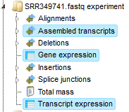
This step distinguishes this workflow from the workflow called “Quantification of RNA-seq with Cufflinks (no de-novo assembly) for FASTQ files”. In the current workflow the transcripts are assembled “de-novo”, whereas in that other workflow the transcripts are taken from the reference Ensembl transcript annotation. Since here it is a “de-novo” reconstruction of exon-intron structure, no known gene or transcript names are given. All transcripts are defined by the tracking_id, like Cuff.1.1 and so on. This allows us to find new transcripts that were not yet discovered and annotated in the reference genome.
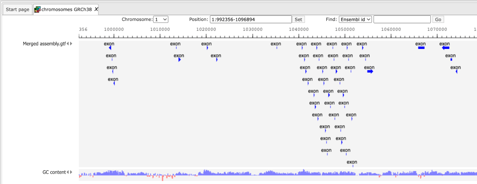
Assembled transcripts merging with Cuffmerge
When you are working with several RNA-seq samples, it becomes necessary to pool the data and assemble them into a comprehensive set of transcripts before proceeding to differential analysis. Cuffmerge, part of the Cufflinks package (https://cufflinks.cbcb.umd.edu/) is essentially a ‘meta-assembler’ — it treats the assembled transfrags the way Cufflinks treats reads, merging them together parsimoniously. Output is a Merged assembly track.
Differential analysis with Cuffdiff
The next step of the workflow is performed by Cuffdiff, part of the Cufflinks package (https://cufflinks.cbcb.umd.edu/), which calculates expression in two or more samples and tests the statistical significance of each observed change in expression between them. Cuffdiff allows supplying multiple technical or biological replicate sequencing libraries per condition. With multiple replicates, Cuffdiff learns how read counts vary for each gene across the replicates and uses these variance estimates to calculate the significance of observed changes in expression.
Cuffdiff reports the following 11 output files:
Detect differentially expressed gene (DEG)
In order to perform further analyses of the results of the workflow Quantification of RNA-seq with Cufflinks for FASTQ files it is recommended to join all resulting gene tables into one table using the function “Join several tables” of the platform. The joint table can be used for detection of differentially expressed genes using the Limma or EBarrays functions.
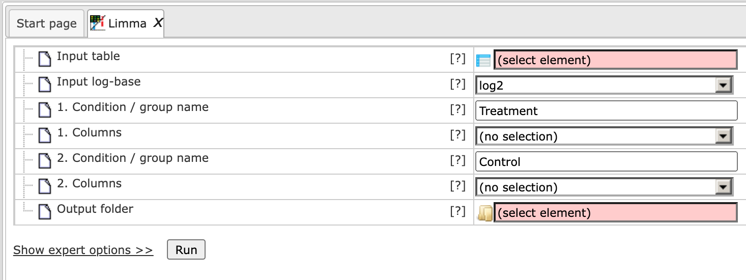
It should be noted here that to perform a Limma or EBarray analysis of the RNA-Seq data you should select the option Unnormalized counts in the input field Input log-base for either of these two methods, as shown below for Limma.
Estimate differential expression using Linear Models for MicroArrays (LIMMA)
Limma estimates differential expression between specified conditions / groups.
This tool provides an interface for the popular and comprehensive Limma package. The platform tool computes differential expression between up to five conditions / groups. The groups consist of columns of a data table that contains normalized measurement values, e.g. from a normalized microarray experiment. Furthermore, one can estimate differential expression for normalized or un-normalized count data as derived from RNA-seq experiments.
All possible contrasts between groups are considered and their output is stored in a common folder. Conditions are compared in the specified order from first to fifth. E.g. given conditions named A, B and C, the output will contain the contrasts AvsB, AvsC and BvsC.
It is necessary to provide a unique name for each group. Also, at least two data columns are required per group.
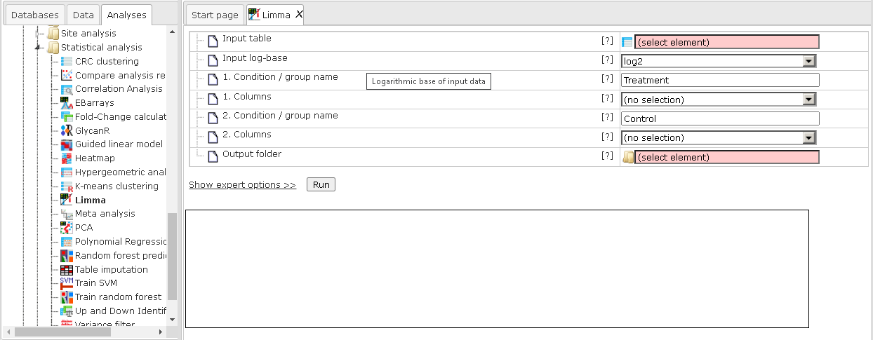
The input parameters for Limma are described in the following.
Input table: This table contains the columns to analyze.
Input log-base: Here you can specify the scale of the input data. If the log-base is log2, the tool will use the data values as is. If your data are from RNA-seq, you can select Normalized counts or Unnormalized counts.
1-5. Condition / group name: One can specify up to five groups of columns. Please note that unnamed groups are not considered; a name is not assigned automatically.
1-5. Columns: These fields contain the selected columns. Please note that column selections are not considered without a corresponding name. Columns can only be specified once and there need to be two columns per group.
Output folder: The output folder will contain one output file for each pair of conditions.
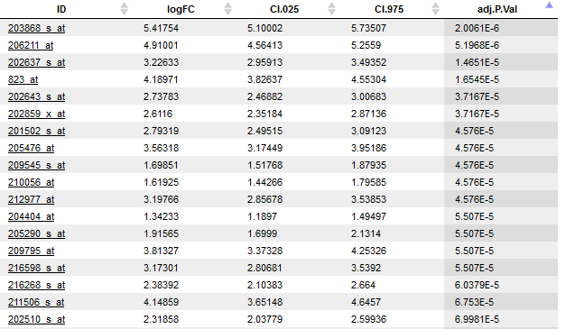
An example output table is shown at the end of this section. Its columns are explained in the following. Those highlighted in bold are shown in the default view. The other columns can be included on demand via the Columns tab of the lower right panel (available with opened output table).
logFC: Fold change (log)
CI.025: Fold change (Lower confidence interval)
CI.975: Fold change (Upper confidence interval)
AveExpr: Average log2-expression for the probe over all arrays
t: Moderated T-statistic
P.Value: P-value Differential expression
adj.P.Val: Adjusted P-value (Benjamini-Hochberg)
B: Log-odds that the gene / probe presents differential expression
Reference:
Smyth, G. K. (2005). Limma: linear models for microarray data. In:
Bioinformatics and Computational Biology Solutions using R and Bioconductor. R.
Gentleman, V. Carey, S. Dudoit, R. Irizarry, W. Huber (eds), Springer, New York,
2005.
Estimate differential expression by the gene expression mixture model of EBarrays
EBarrays estimates differential expression between specified conditions / groups.
This tool provides for differential expression analysis using the EBarrays package. The platform tool can compare up to five conditions / groups. The groups consist of columns of a data table that contains normalized measurement values, e.g. from a normalized microarray experiment.
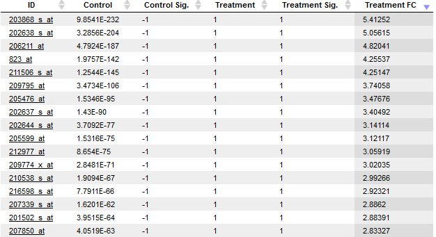
EBarrays sets up a mixture model matching the specified groups. Differential expression is identified when components for a pattern describe the distribution of measurement values well. Then probe / gene values in the corresponding group were significantly different from their values in the other groups. This is reflected by high posterior probabilities in the column named after that group.
The package estimates a critical posterior probability cutoff for the given FDR level on the basis of the fitted mixture model. Probes / genes exceeding this cutoff in some condition / group are indicated by a value of 1 (instead of -1) in the output column named “condition name Sig”. Hence, to isolate the targets differentially expressed in a condition of interest, e.g. condition named “treatment”, filter the table for all rows with a value of 1 in the column “treatment Sig”. The direction of differential expression can be derived from the fold change column “condition name FC”, which contains the log2-fold changes.
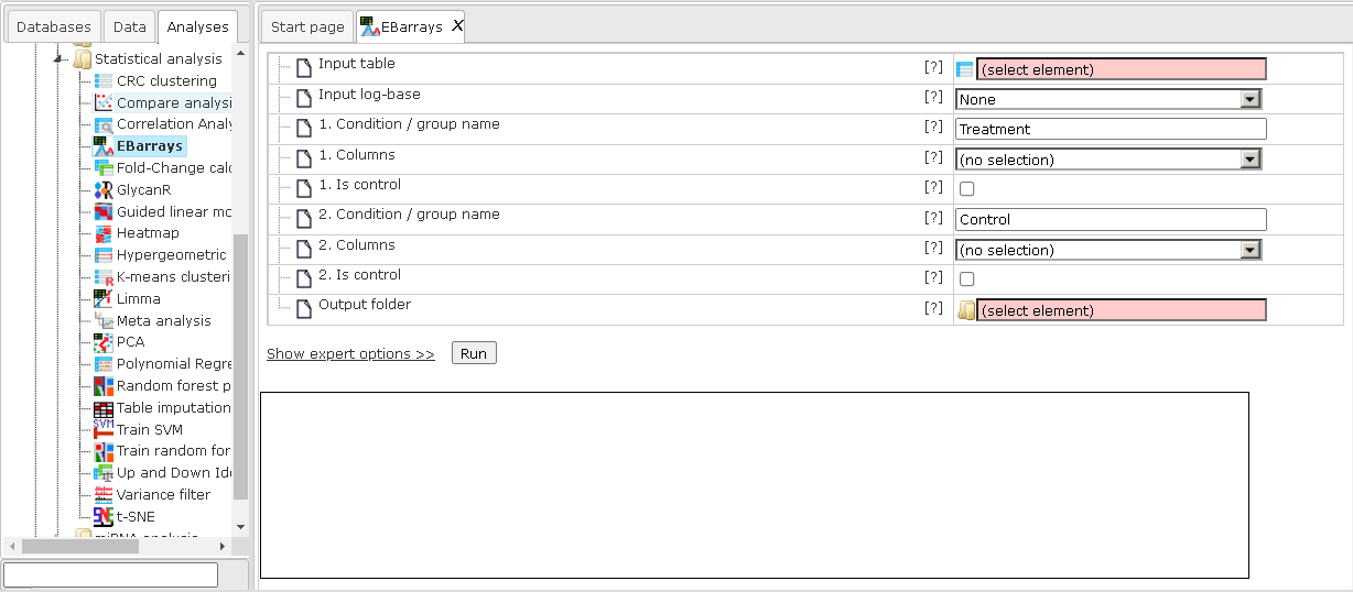
The input parameters for EBarrays are described in the following.
Input table: This table contains the columns to analyze.
Input log-base: Here you can specify the scale of the input data. If the log-base is none, the tool will use the data values as is. If your data are from RNA-seq, you can select Normalized counts or Unnormalized counts.
1-5. Condition / group name: One can specify up to five groups of columns. Please note that unnamed groups are not considered; a name is not assigned automatically. Fields for the first two groups need to be set.
1-5. Columns: These fields contain the selected columns. Please note that column selections are not considered without a corresponding name. Columns can only be specified once and there need to be two columns per group. Fields for the first two groups need to be set.
1-5. Is control: Use this field to mark the control column group. One such group is required.
Output folder: The output folder will contain one output file for each pair of conditions.
It is necessary to provide a unique name for each group. Also, at least two data columns are required per group and one group needs to be marked as a control group.
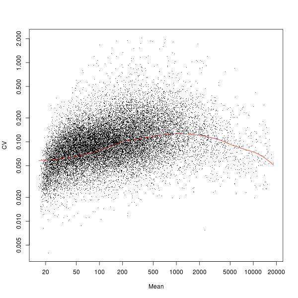
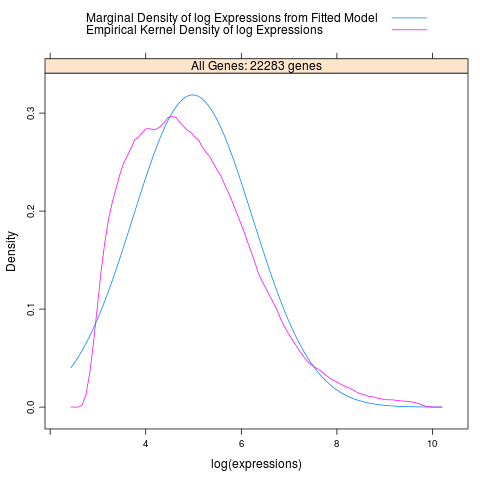
Besides the main output table containing differential expression estimates for each probe / gene, EBarrays provides two diagnostic plots named EBarrays CCV and EBarrays Marginal fit. These plots enable a judgment about whether assumptions of the approach hold and how well the fitted model represents the data (please refer to the documentation of the EBarrays Bioconductor package for further details). Examples of an output table, a CCV plot and a Marginal fit plot are shown at the end of this section.
Reference:
Kendziorski, C.M., Newton, M.A., Lan, H., Gould, M.N. (2003). On parametric
empirical Bayes methods for comparing multiple groups using replicated gene
expression profiles. Statistics in Medicine 22:3899-3914.