Epigenomics
Site search with TRANSFAC(R)
Site search in a single interval list
This workflow helps to map putative TFBSs on peaks calculated from your
ChIP-seq data. Site search is done with the help of the TRANSFAC® library of
positional weight matrices, PWMs, using the pre-computed profile
vertebrate_non_redundant_minSUM. This is described in detail in Chip-seq section.
Site search in multiple interval sets
This workflow is designed to search for TFBSs in DNA sequences identified by the ChIP-seq approach, for multiple datasets. This workflow is described in detail in Chip-seq section.
Search for composite modules
Search for composite modules with TRANSFAC®
This workflow finds pairs of TFBSs that discriminate between two tracks, the Yes and the No track. As the Yes track, ChIP-seq peaks or intervals identified in analyses for histone modifications, or any other genomic fragments, can be considered. This workflow is described in detail in Chip-seq section.
Search for discriminative sites with TRANSFAC® (MEALR)
The tool MEALR finds combinations of TFBS matrices that discriminate between two sets of sequences (denoted as Yes and No sets). The Yes set may consist of genomic regions identified in a ChIP-seq experiment. No sequences are often other non-coding genomic regions not overlapping with the peaks.
MEALR differs from other tools in the following points.
No cutoff or threshold is used on matrix scores to determine potential binding sites. Instead, MEALR calculates threshold-free sequence scores.
MEALR builds a discriminative model for classification which is well-established and widely applied in statistical analysis called Sparse Logistic Regression. The model consists of a linear model that estimates the probability that a sequence belongs to the Yes set based on its binding site features.
The sparseness constraint enables MEALR to select a subset of matrices relevant for classification of Yes and No sequences from a possibly large matrix library. Therefore MEALR’s output differs from other tools by presenting a focused set of matrices.
While other site enrichment tools provided in the platform evaluate enrichment separately for each matrix, the model used in MEALR assesses the importance of matrices for discrimination in combination with other matrices of the library. Therefore, MEALR suggests (linear) combinations of transcription factor motifs.
MEALR calculates the score x of the ith sequence according to the kth matrix as $$x_{\text{ik}} = \log(\frac{1}{{\ L}}{i}\sum{w_{i}^{}{\ \exp}}\left( S_{w} \right))$$, where Sw is the log-odds score of the wth window of matrix length. Each sequence is therefore associated with a vector of scores, one from each matrix, and a class (Yes, No).
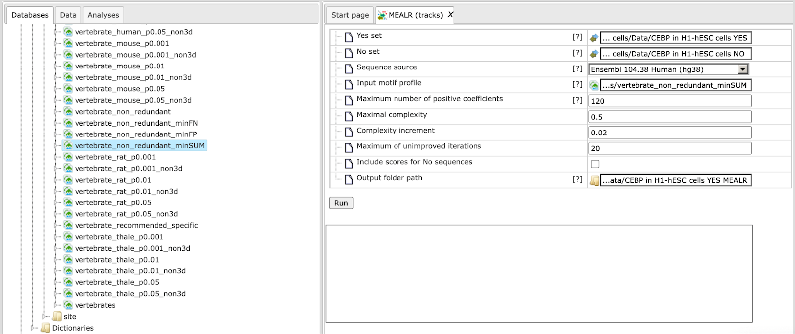
Let us present an example analysis for a ChIP-seq data set consisting of 500 peak regions and 1000 sequences randomly sampled from regulatory regions across the human genome. The figure below depicts the input mask of the analysis tool.
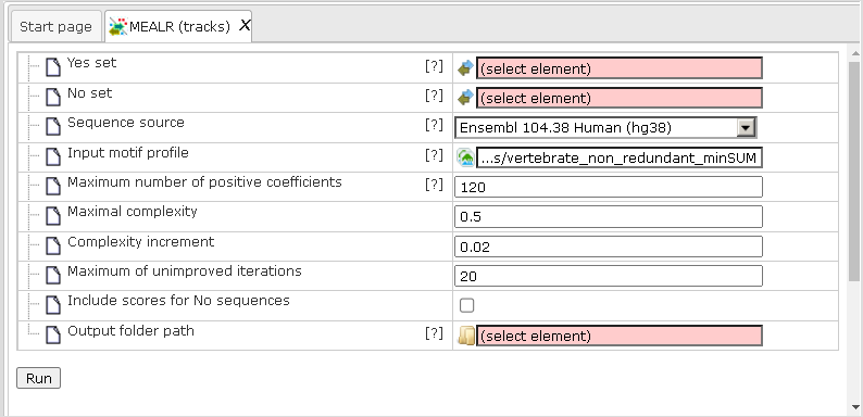
Yes set: This is the set of sequence intervals that you want to analyze, for example these can be ChIP-seq peak regions.
No set: This is the set of background intervals (control set).
Sequence source: Both Yes and No track need to refer to a common source, such as a genome, as specified by this parameter. Note that you can apply a custom source, e.g. a specifically uploaded genome. Clicking on the “Custom” option will open a new field to choose the custom sequence source.
Input motif profile: The profile lists the PWMs (motifs) that are used to assign scores to Yes and No sequences. By default, this field is set to the profile last applied in your workspace. Note that cutoffs in the profile are ignored, because MEALR calculates whole sequence scores.
Output path: In this field you select a path in the workspace to store the output table.
The steps of an analysis can be described as follows:
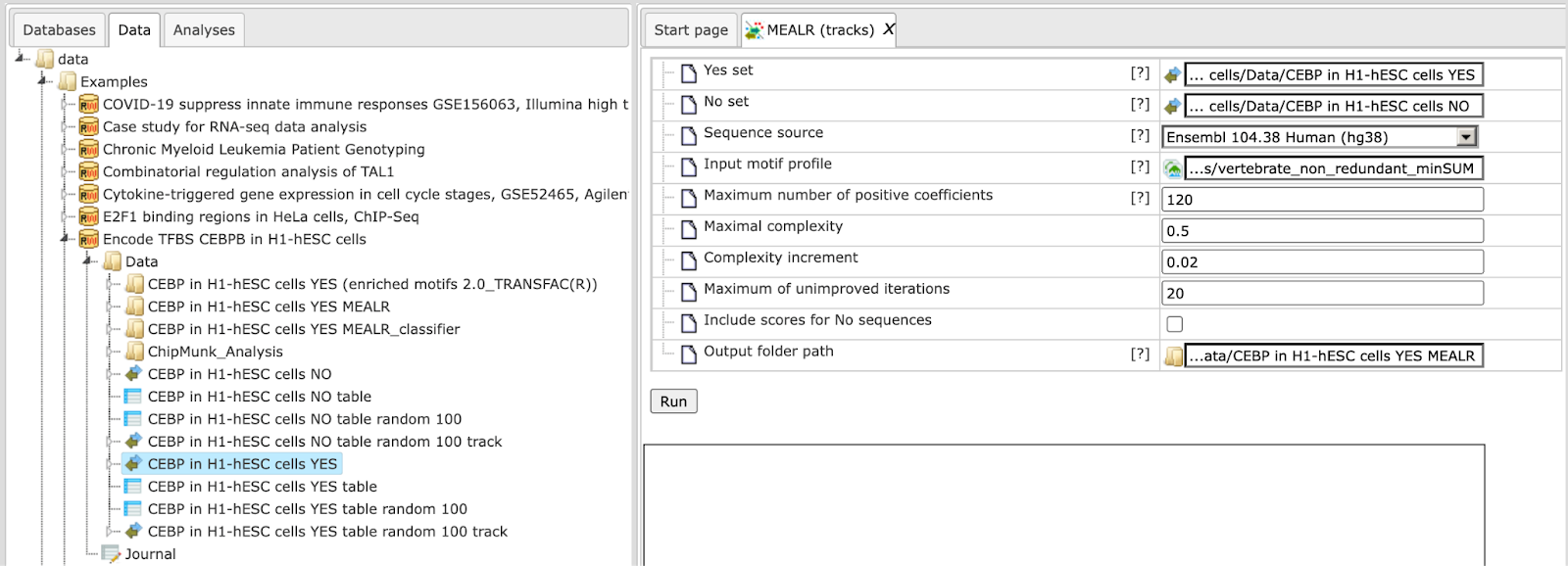
Step 1. Input Yes set from the tree. As usual, you can drag-and-drop. Here, the set of YES intervals from the Example folder is used as input, highlighted blue on the screenshot below:
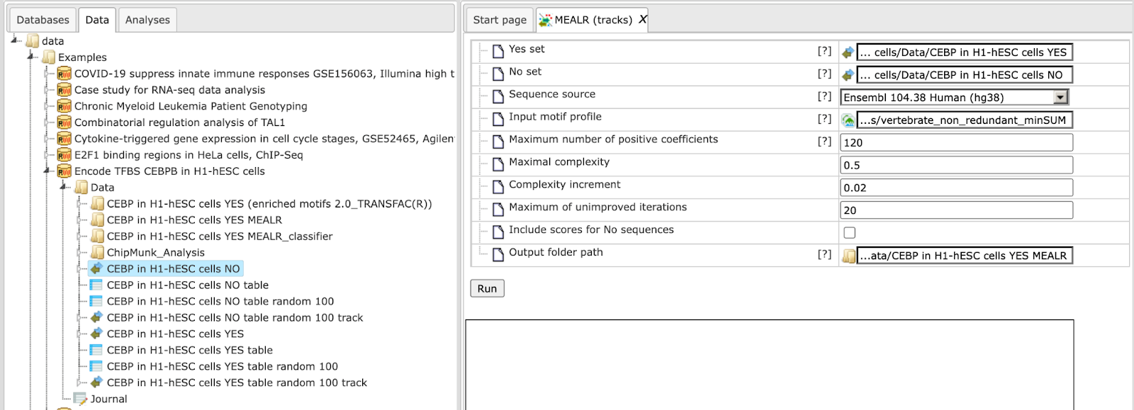
Step 2. Input No set (drag-and-drop). Our example uses the set of NO intervals:
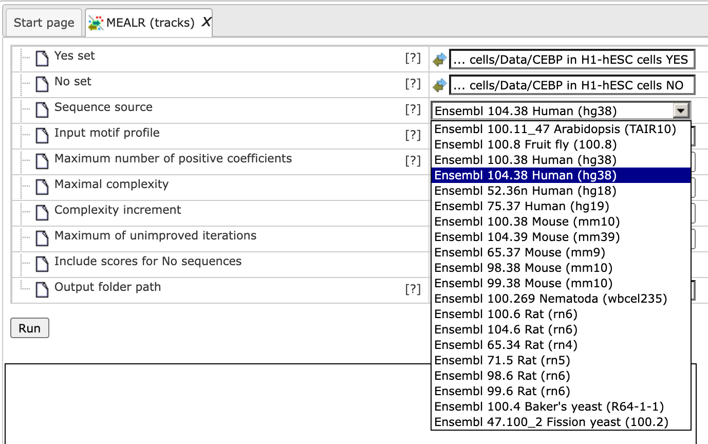
Step 3. The sequence source should be set automatically upon specifying the interval sets. If not select the corresponding sequence source from the pull-down list:
Step 4. Select the TRANSFAC® or GTRD profile from the available profiles. In this example, we select the latest TRANSFAC® profile named “vertebrate_non_redundant”:
Step 5. Edit the output path. After setting the Yes set, a default output path is suggested. The Example folder may not be writable for your account requiring selection of an alternative such as one of your own projects. A different selection can be made easily by clicking on the field.
Clicking the [Run] button will invoke the analysis. The summary table is automatically opened in a new tab when the analysis is completed. Here is a
part of the output for our example:
is automatically opened in a new tab when the analysis is completed. Here is a
part of the output for our example:
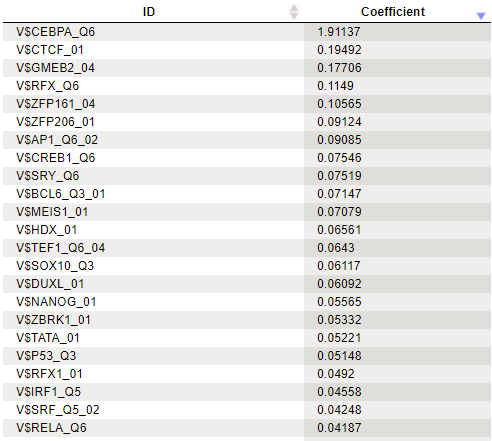
A row of the output table contains a matrix identifier and its logistic regression coefficient. The larger the coefficient value, the more important the corresponding matrix was for discriminating between Yes and No sequences. In our example, three of the five top matrices represent members of the transcription factor subfamily C/EBP.