Workflows
Common
Analyze multiple BAM files to detect DEGs
This workflow is designed to analyze a biological experiment with two conditions (for example patients with a disease and healthy patients). The workflow will use BAM tracks to assign the sequence reads to genomic features, in this case genes. Finally using statistics to determine differentially expressed genes between the two input conditions.
✨ [Open](https://platform.genexplain.com/bioumlweb/#de=analyses/Workflows/Common /Analyze%20multiple%20BAM%20files%20to%20detect%20DEGs) the workflow in the user interface.✨
The following list gives an overview of all input parameters used in this workflow:
Parameter |
Description |
|---|---|
Experiment BAM files |
Two or several BAM files |
Control BAM files |
Two or several BAM files |
ReferenceEnsembl |
Select your reference genome |
Results folder |
Name and location of outputs |
Two or several BAM files can be submitted in the input field Experiment BAM files as one condition in your experiment like disease. An example BAM file can be found here.
Two or several single-end FASTQ files can be submitted in the input field Control BAM files as a second condition in your experiment like healthy. An example FASTQ file can be found here.
You can drag and drop the input BAM files from your data project within the tree area or you may click into the input field [0] and a new window will be opened, where you can select your input BAM files. You may also select several FASTQ files at once using the Control button of your computer.
As reference genome the most recent Ensembl human genome (Ensembl GRCh38; hg38) is used and set as default. for the workflow run. You can select the reference genome of your paired library from the drop-down list ReferenceEnsembl to your needs.
The outputs of counting genes are saved in two tables: one file contains the counts (result example) and the other a count summary of the counting procedure (result example).
The last step of the workflow performs a differential expression analysis on raw counts with limma-voom:
voom: Prepares RNA-Seq data for linear modelling by transforming count data to log2-counts per million (logCPM), estimating the mean-variance relationship and computing appropriate observation-level weights.
lmFit: Fits a linear model using weighted least squares for each gene.
eBayes: Assesses differential expression using moderated t-statistic.
A normalization of the data is done by the limma-voom method, which applies calcNormFactors from the edgeR package and calculates normalization factors to scale the raw library sizes. TMM normalization method is used - the weighted trimmed mean of M-values (to the reference) proposed by Robinson and Oshlack (2010), where the weights are from the delta method on Binomial data.
A result folder of the limma-voom analysis is generated and contains several tables. All raw counts from all conditions are fully joined in a common table (result example), further filtering to exclude low expressed genes (less than 10 counts) generates another table (result example).
After normalization the prepared table (result example) is used to determine DEGs as a final table (result example) with two filtered tables of up-regulated (result example) and down-regulated genes (result example) as well as non-regulated genes (result example). A plot is generated, which compares unnormalized and normalized data (result example).
Following filter conditions are used:
Up-regulated genes: logFC > 0.5 && P-value < 0.05
Down-regulated genes: logFC < -0.5 && P-value < 0.05
Non-regulated genes: select middle percentage of DEGs (min 100 & max 1000)
All output results can be exported to your local computer.
ChIP-Seq - Identify and classify target genes
This workflow is designed to identify target genes of ChIP-seq peaks and perform functional classification of these targets with mapping to different ontologies: Gene Ontology biological processes, Gene Ontology cellular components, Gene Ontology molecular function, Transcription factor classification (TFclass), Reactome pathways, and HumanCyc pathways. In parallel, the target gene list is subjected to a cluster analysis and clusters are visualized based on the GeneWays protein interaction network database.
✨ Open the workflow in the user interface.✨
The following list gives an overview of all input parameters used in this workflow:
Parameter |
Description |
|---|---|
Input track |
ChIP-Seq track |
Species |
Define the species of your data |
AnnotationSource |
Ensembl annotation source file |
Results folder |
Name and location of outputs |
Normalized data with Affymetrix probeset IDs can be submitted in the input fields Input track (input example).
You can drag and drop the ChIP-seq track from your data project within the tree area or you may click into the input field (select element) and a new window will be opened, where you can select your ChIP-seq track.
You need to select the biological species of your data in the field Species by choosing the required one from the drop-down menu.
For gene annotation the most recent Ensembl database is used and set as default. for the workflow run. You can adapt the database version in the field AnnotationSource to your needs.
In the first part of the workflow the ChIP-seq track is mapped and converted to the target gene fragments with a 5’ region and 3’ region size of 1000bp. The resulting Ensembl gene list is annotated with additional gene information (gene descriptions, gene symbols, and species) via the Annotate table method. Another Entrez gene table is generated with the Convert table method, which is further needed for the cluster analysis as input.
The method Cluster by shortest path created networks based on the protein reactions annotated in the GeneWays database. The algorithm included as many target genes as possible from the previously created Entrez gene list. The proteins that result from the respective genes, were allowed to be a maximum of two reactions apart. The resulting networks out of the clusters are visualized and given in the output.
In the second part of the workflow the list of Ensembl target genes is mapped to the following functional classifications:
Gene Ontology (biological process)
Gene Ontology (cellular component)
Gene Ontology (molecular function)
HumanCyc pathways
Reactome pathways
Transcription factor classification (TFclass)
At least two target genes must be mapped into one group (e.g. one GO term, one pathway) and a P-value threshold lower 0.05 is given for each group.
A result folder is generated and contains the two resulting target gene lists (Ensembl ID format (result example) and Entrez ID format (result example), all resulting tables of the functional classification mapping (result example), and a subfolder with the clustering output (result example).
All output results can be exported to your local computer.
Compute differentially expressed genes (Affymetrix probes)
This workflow is designed to identify differentially expressed genes from an experiment data set compared to a control data set.
✨ Open the workflow in the user interface.✨
The following list gives an overview of all input parameters used in this workflow:
Parameter |
Description |
|---|---|
Experiment normalized |
Table with normalized Affymetrix data |
Control normalized |
Table with normalized Affymetrix data |
Probe type |
Specify the Affymetrix Chip type |
Species |
Define the species of your data |
AnnotationSource |
Ensembl annotation source file |
Results folder |
Name and location of outputs |
Normalized data with Affymetrix probeset IDs can be submitted in the input fields Experiment normalized (input example) and Control normalized (input example). Such normalized files are the output of the method Normalize Affymetrix experiment and control.
You can drag and drop normalized data from your data project within the tree area or you may click into the input field (select element) and a new window will be opened, where you can select your normalized data.
Please select the Affymetrix Chip you have used in your experiment or your data corresponds to in the field Probe type by selecting the correct one from the drop-down menu. Support for the following probe types from Affymetrix Chips are given:
Affymetrix
Affymetrix ST
Affymetrix HG-U133+ PM
Affymetrix HuGene-2_1-st
Affymetrix HuGene-2_0-st
Affymetrix RaGene-2_0-st
Affymetrix miRNA-1_0
Affymetrix miRNA-2_0
Affymetrix miRNA-3_0
Affymetrix miRNA-4_0
Affymetrix miRNA-4_1
You need to select the biological species of your data in the field Species by choosing the required one from the drop-down menu.
For gene annotation the most recent Ensembl database is used and set as default. for the workflow run. You can adapt the database version in the field AnnotationSource to your needs.
In the first step the up- and down-regulated probes are identified and log fold change values are calculated for all probe IDs. This method applies Student’s T-test and calculates p-values, thus the number of data points should be at least three for each experiment data set and control data set. A histogram with the log fold change distribution from the whole experiment is drawn and given in an output image file.
In addition the results are filtered by different conditions in parallel applying the Filter table method, to identify up-regulated, down-regulated, and non-changed Affymetrix probeset IDs. The filtering criteria are set as follows:
For up-regulated probes: LogFoldChange > 0.5 and -log(P-value) > 3
For down- regulated probes: LogFoldChange < -0.5 and -log(P-value) < -3
For non-changed genes : LogFoldChange < 0.002 and LogFoldChange > -0.002
The resulting tables of up-regulated, down-regulated, and non-changed Affymetrix probeset IDs are converted into Ensembl gene tables with the Convert table method and annotated with additional gene information (gene descriptions, gene symbols, and species) via the Annotate table method.
A result folder is generated and contains all tables, the histogram and a summary HTML report (report example). All output results can be exported to your local computer.
All output results can be exported to your local computer.
Compute differentially expressed genes (Agilent Tox probes)
This workflow is designed to identify differentially expressed genes from an experiment data set compared to a control data set.
✨ Open the workflow in the user interface.✨
The following list gives an overview of all input parameters used in this workflow:
Parameter |
Description |
|---|---|
Experiment normalized |
Table with normalized Agilent tox data |
Control normalized |
Table with normalized Agilent tox data |
Species |
Define the species of your data |
AnnotationSource |
Ensembl annotation source file |
Results folder |
Name and location of outputs |
Normalized data with Affymetrix probeset IDs can be submitted in the input fields Experiment normalized and Control normalized. Such normalized files are the output of the method Normalize Affymetrix experiment and control.
[Agil tox normalized]:
[Agil tox con normalized]:
You can drag and drop normalized data from your data project within the tree area or you may click into the input field (select element) and a new window will be opened, where you can select your normalized data.
You need to select the biological species of your data in the field Species by choosing the required one from the drop-down menu.
For gene annotation the most recent Ensembl database is used and set as default. for the workflow run. You can adapt the database version in the field AnnotationSource to your needs.
In the first step the up- and down-regulated probes are identified and log fold change values are calculated for all probe IDs. This method applies Student’s T-test and calculates p-values, thus the number of data points should be at least three for each experiment data set and control data set. A histogram with the log fold change distribution from the whole experiment is drawn and given in an output image file.
In addition the results are filtered by different conditions in parallel applying the Filter table method, to identify up-regulated, down-regulated, and non-changed Agilent tox probeset IDs. The filtering criteria are set as follows:
For up-regulated probes: LogFoldChange > 0.5 and -log(P-value) > 3
For down- regulated probes: LogFoldChange < -0.5 and -log(P-value) < -3
For non-changed genes : LogFoldChange < 0.002 and LogFoldChange > -0.002
The resulting tables of up-regulated, down-regulated, and non-changed Agilent tox probeset IDs are converted into Ensembl gene tables with the Convert table method and annotated with additional gene information (gene descriptions, gene symbols, and species) via the Annotate table method.
A result folder is generated and contains all tables, the histogram and a summary HTML report ([report example][Agil tox report]).
All output results can be exported to your local computer.
Compute differentially expressed genes (Agilent probes)
This workflow is designed to identify differentially expressed genes from an experiment data set compared to a control data set.
✨Open the workflow in the user interface.✨
The following list gives an overview of all input parameters used in this workflow:
Parameter |
Description |
|---|---|
Experiment normalized |
Table with normalized Agilent data |
Control normalized |
Table with normalized Agilent data |
Species |
Define the species of your data |
AnnotationSource |
Ensembl annotation source file |
Results folder |
Name and location of outputs |
Normalized data with Agilent probeset IDs can be submitted in the input fields Experiment normalized (input example) and Control normalized (input example). Such normalized files are the output of the method Normalize Agilent experiment and control.
You can drag and drop normalized data from your data project within the tree area or you may click into the input field (select element) and a new window will be opened, where you can select your normalized data.
You need to select the biological species of your data in the field Species by choosing the required one from the drop-down menu.
For gene annotation the most recent Ensembl database is used and set as default. for the workflow run. You can adapt the database version in the field AnnotationSource to your needs.
In the first step the up- and down-regulated probes are identified and log fold change values are calculated for all probe IDs. This method applies Student’s T-test and calculates p-values, thus the number of data points should be at least three for each experiment data set and control data set. A histogram with the log fold change distribution from the whole experiment is drawn and given in an output image file.
In addition the results are filtered by different conditions in parallel applying the Filter table method, to identify up-regulated, down-regulated, and non-changed Agilent probeset IDs. The filtering criteria are set as follows:
For up-regulated probes: LogFoldChange > 0.5 and -log(P-value) > 3
For down- regulated probes: LogFoldChange < -0.5 and -log(P-value) < -3
For non-changed genes : LogFoldChange < 0.002 and LogFoldChange > -0.002
The resulting tables of up-regulated, down-regulated, and non-changed Agilent probeset IDs are converted into Ensembl gene tables with the Convert table method and annotated with additional gene information (gene descriptions, gene symbols, and species) via the Annotate table method.
A result folder is generated and contains all tables, the histogram and a summary HTML report (report example).
All output results can be exported to your local computer.
Compute differentially expressed genes (Illumina probes)
This workflow is designed to identify differentially expressed genes from an experiment data set compared to a control data set.
✨Open the workflow in the user interface.✨
The following list gives an overview of all input parameters used in this workflow:
Parameter |
Description |
|---|---|
Experiment normalized |
Table with normalized Illumina data |
Control normalized |
Table with normalized Illumina data |
Species |
Define the species of your data |
AnnotationSource |
Ensembl annotation source file |
Results folder |
Name and location of outputs |
Normalized data with Illumina probeset IDs can be submitted in the input fields Experiment normalized (input example) and Control normalized (input example). Such normalized files are the output of the method Normalize Illumina experiment and control.
You can drag and drop normalized data from your data project within the tree area or you may click into the input field (select element) and a new window will be opened, where you can select your normalized data.
You need to select the biological species of your data in the field Species by choosing the required one from the drop-down menu.
For gene annotation the most recent Ensembl database is used and set as default. for the workflow run. You can adapt the database version in the field AnnotationSource to your needs.
In the first step the up- and down-regulated probes are identified and log fold change values are calculated for all probe IDs. This method applies Student’s T-test and calculates p-values, thus the number of data points should be at least three for each experiment data set and control data set. A histogram with the log fold change distribution from the whole experiment is drawn and given in an output image file.
In addition the results are filtered by different conditions in parallel applying the Filter table method, to identify up-regulated, down-regulated, and non-changed Illumina probeset IDs. The filtering criteria are set as follows:
For up-regulated probes: LogFoldChange > 0.5 and -log(P-value) > 3
For down- regulated probes: LogFoldChange < -0.5 and -log(P-value) < -3
For non-changed genes : LogFoldChange < 0.002 and LogFoldChange > -0.002
The resulting tables of up-regulated, down-regulated, and non-changed Illumina probeset IDs are converted into Ensembl gene tables with the Convert table method and annotated with additional gene information (gene descriptions, gene symbols, and species) via the Annotate table method.
A result folder is generated and contains all tables, the histogram and a summary HTML report (report example).
All output results can be exported to your local computer.
Compute differentially expressed genes using EBarrays
This workflow is designed to estimate differentially expressed genes with EBarrays between specified conditions / groups.
✨ Open the workflow in the user interface.✨
The following list gives an overview of all input parameters used in this workflow:
Parameter |
Description |
|---|---|
Input table |
Table with normalized data |
Probe type |
Specify the Affymetrix Chip type |
Species |
Define the species of your data |
AnnotationSource |
Ensembl annotation source file |
Control_group |
Enter control group name without spaces |
Columns_control |
Select columns of control samples |
Condition_1_group |
Enter Condition 1 group name without spaces |
Columns_condition_1 |
Select columns of condition 1 samples |
Condition_2_group |
Enter Condition 2 group name without spaces |
Columns_condition_2 |
Select columns of condition 2 samples |
Condition_3_group |
Enter Condition 3 group name without spaces |
Columns_condition_3 |
Select columns of condition 3 samples |
Condition_4_group |
Enter Condition 4 group name without spaces |
Columns_condition_4 |
Select columns of condition 4 samples |
Results folder |
Name and location of outputs |
Normalized data from the microarray experiment can be submitted in the input field Input table (input example). Such a normalized file is the output of the method Affymetrix normalization.
You can drag and drop normalized data from your data project within the tree area or you may click into the input field (select element) and a new window will be opened, where you can select your normalized data.
You need to select the biological species of your data in the field Species by choosing the required one from the drop-down menu.
For gene annotation the most recent Ensembl database is used and set as default. for the workflow run. You can adapt the database version in the field AnnotationSource to your needs.
The workflow compares up to five conditions / groups. It is necessary to provide a unique name for each group. Also, at least two data columns are required per group and the first group is marked as a control group.
Besides the main output tables containing differential expression estimates for each gene, EBarrays provides two diagnostic plots named EBarrays CCV and EBarrays Marginal fit. These plots enable a judgment about whether assumptions of the approach hold and how well the fitted model represents the data.EBarrays estimates a critical posterior probability cut-off for the given FDR level on the basis of the fitted mixture model. Probes / genes exceeding this cut-off in some condition / group are indicated by a value of 1 (instead of -1) in the output column named “condition name Sig”. The resulting tables with up- and down-regulated genes are filtered with the following conditions:
For up-regulated genes: log2-fold changes > 0.5 and cut-off FDR level < 0.05
For down-regulated genes: log2-fold changes < -0.5 and cut-off FDR level < 0.05
A result folder is generated and contains one folder with unfiltered EBarrays results (result example), one folder with the diagnostic plots (result example) and all filtered gene tables with significantly differentially expressed genes for all condition groups compared to the control group.
All output results can be exported to your local computer.
Compute differentially expressed genes using Hypergeometric test (Affymetrix probes)
This workflow is designed to identify differentially expressed genes from an experiment data set compared to a control data set.
✨ Open the workflow in the user interface.✨
The following list gives an overview of all input parameters used in this workflow:
Parameter |
Description |
|---|---|
Experiment normalized |
Table with normalized Affymetrix data |
Control normalized |
Table with normalized Affymetrix data |
Probe type |
Specify the Affymetrix Chip type |
Species |
Define the species of your data |
AnnotationSource |
Ensembl annotation source file |
Results folder |
Name and location of outputs |
Normalized data with Affymetrix probeset IDs can be submitted in the input fields Experiment normalized (input example) and Control normalized (input example). Such normalized files are the output of the method Normalize Affymetrix experiment and control.
You can drag and drop normalized data from your data project within the tree area or you may click into the input field (select element) and a new window will be opened, where you can select your normalized data.
Please select the Affymetrix Chip you have used in your experiment or your data corresponds to in the field Probe type by selecting the correct one from the drop-down menu. Support for the following probe types from Affymetrix Chips are given:
Affymetrix
Affymetrix ST
Affymetrix HG-U133+ PM
Affymetrix HuGene-2_1-st
Affymetrix HuGene-2_0-st
Affymetrix RaGene-2_0-st
Affymetrix miRNA-1_0
Affymetrix miRNA-2_0
Affymetrix miRNA-3_0
Affymetrix miRNA-4_0
Affymetrix miRNA-4_1
You need to select the biological species of your data in the field Species by choosing the required one from the drop-down menu.
For gene annotation the most recent Ensembl database is used and set as default. for the workflow run. You can adapt the database version in the field AnnotationSource to your needs.
In the first step the up- and down-regulated probes are identified and log fold change values are calculated for all probe IDs. The p-value is calculated by hypergeometric analysis
Paper
Y. V. Kondrakhin, R. N. Sharipov, A. E. Kel, F. A. Kolpakov. (2008) Identification of Differentially Expressed Genes by Meta-Analysis of Microarray Data on Breast Cancer, In Silico Biology, 8: 383-411. link
A histogram with the log fold change distribution from the whole experiment is drawn and given in an output image file (output example). If you have just two or even one sample for your experiment and for your control (e.g. one CEL file in experiment and one CEL file in control), you can apply hypergeometric analysis to calculate DEGs. In contrast to the t-test which requires at least three sample replicates, hypergeometric analysis can make calculations for two and even one sample.
In addition the results are filtered by different conditions in parallel to identify up-regulated, down-regulated, and non-changed Affymetrix probeset IDs. The filtering criteria are set as follows:
For up-regulated probes: LogFoldChange > 0.5 and -log(P-value) > 3
For down- regulated probes: LogFoldChange < -0.5 and -log(P-value) < -3
For non-changed genes : LogFoldChange < 0.002 and LogFoldChange > -0.002
The resulting tables of up-regulated, down-regulated, and non-changed Affymetrix probeset IDs are converted into Ensembl gene tables with the Convert table method and annotated with additional gene information (gene descriptions, gene symbols, and species) via the Annotate table method (output example).
A result folder is generated and contains all tables, the histogram and a summary HTML report (report example).
All output results can be exported to your local computer.
Compute differentially expressed genes using Hypergeometric test (Agilent probes)
This workflow is designed to identify differentially expressed genes from an experiment data set compared to a control data set.
✨ Open the workflow in the user interface.✨
The following list gives an overview of all input parameters used in this workflow:
Parameter |
Description |
|---|---|
Experiment normalized |
Table with normalized Agilent data |
Control normalized |
Table with normalized Agilent data |
Species |
Define the species of your data |
AnnotationSource |
Ensembl annotation source file |
Results folder |
Name and location of outputs |
Normalized data with Agilent probeset IDs can be submitted in the input fields Experiment normalized (input example) and Control normalized (input example). Such normalized files are the output of the method Normalize Agilent experiment and control.
You can drag and drop normalized data from your data project within the tree area or you may click into the input field (select element) and a new window will be opened, where you can select your normalized data.
You need to select the biological species of your data in the field Species by choosing the required one from the drop-down menu.
For gene annotation the most recent Ensembl database is used and set as default. for the workflow run. You can adapt the database version in the field AnnotationSource to your needs.
In the first step the up- and down-regulated probes are identified and log fold change values are calculated for all probe IDs. The p-value is calculated by hypergeometric analysis.
Paper
Y. V. Kondrakhin, R. N. Sharipov, A. E. Kel, F. A. Kolpakov. (2008) Identification of Differentially Expressed Genes by Meta-Analysis of Microarray Data on Breast Cancer, In Silico Biology, 8: 383-411. link
A histogram with the log fold change distribution from the whole experiment is drawn and given in an output image file. If you have just two or even one sample for your experiment and for your control (e.g. one CEL file in experiment and one CEL file in control), you can apply hypergeometric analysis to calculate DEGs. In contrast to the t-test which requires at least three sample replicates, hypergeometric analysis can make calculations for two and even one sample.
In addition the results are filtered by different conditions in parallel applying the Filter table method, to identify up-regulated, down-regulated, and non-changed Agilent probeset IDs. The filtering criteria are set as follows:
For up-regulated probes: LogFoldChange > 0.5 and -log(P-value) > 3
For down- regulated probes: LogFoldChange < -0.5 and -log(P-value) < -3
For non-changed genes : LogFoldChange < 0.002 and LogFoldChange > -0.002
The resulting tables of up-regulated, down-regulated, and non-changed Agilent probeset IDs are converted into Ensembl gene tables with the Convert table method and annotated with additional gene information (gene descriptions, gene symbols, and species) via the Annotate table method(output example).
A result folder is generated and contains all tables, the histogram and a summary HTML report (report example).
All output results can be exported to your local computer.
Compute differentially expressed genes using Hypergeometric test (Illumina probes)
This workflow is designed to identify differentially expressed genes from an experiment data set compared to a control data set.
✨ Open the workflow in the user interface.✨
The following list gives an overview of all input parameters used in this workflow:
Parameter |
Description |
|---|---|
Experiment normalized |
Table with normalized Illumina data |
Control normalized |
Table with normalized Illumina data |
Species |
Define the species of your data |
AnnotationSource |
Ensembl annotation source file |
Results folder |
Name and location of outputs |
Normalized data with Agilent probeset IDs can be submitted in the input fields Experiment normalized (input example) and Control normalized (input example). Such normalized files are the output of the method Normalize Illumina experiment and control.
You can drag and drop normalized data from your data project within the tree area or you may click into the input field (select element) and a new window will be opened, where you can select your normalized data.
You need to select the biological species of your data in the field Species by choosing the required one from the drop-down menu.
For gene annotation the most recent Ensembl database is used and set as default. for the workflow run. You can adapt the database version in the field AnnotationSource to your needs.
In the first step the up- and down-regulated probes are identified and log fold change values are calculated for all probe IDs. The p-value is calculated by hypergeometric analysis.
Paper
Y. V. Kondrakhin, R. N. Sharipov, A. E. Kel, F. A. Kolpakov. (2008) Identification of Differentially Expressed Genes by Meta-Analysis of Microarray Data on Breast Cancer, In Silico Biology, 8: 383-411. link
A histogram with the log fold change distribution from the whole experiment is drawn and given in an output image file. If you have just two or even one sample for your experiment and for your control (e.g. one Illumina file in experiment and one Illumina file in control), you can apply hypergeometric analysis to calculate DEGs. In contrast to the t-test which requires at least three sample replicates, hypergeometric analysis can make calculations for two and even one sample.
In addition the results are filtered by different conditions in parallel applying the Filter table method, to identify up-regulated, down-regulated, and non-changed Illumina probeset IDs. The filtering criteria are set as follows:
For up-regulated probes: LogFoldChange > 0.5 and -log(P-value) > 3
For down- regulated probes: LogFoldChange < -0.5 and -log(P-value) < -3
For non-changed genes : LogFoldChange < 0.002 and LogFoldChange > -0.002
The resulting tables of up-regulated, down-regulated, and non-changed Illumina probeset IDs are converted into Ensembl gene tables with the Convert table method and annotated with additional gene information (gene descriptions, gene symbols, and species) via the Annotate table method .
All output results can be exported to your local computer.
Compute differentially expressed genes using Limma
This workflow is designed to estimate differentially expressed genes with limma between specified conditions / groups.
✨ Open the workflow in the user interface.✨
The following list gives an overview of all input parameters used in this workflow:
Parameter |
Description |
|---|---|
Input table |
Table with normalized data |
Probe type |
Please specify the microarray chip type or select Illumina gene count table |
Species |
Define the species of your data |
AnnotationSource |
Ensembl annotation source file |
Condition_1 |
Enter Condition 1 group name without spaces |
1_Columns |
Select columns of condition 1 samples |
Condition_2 |
Enter Condition 2 group name without spaces |
2_Columns |
Select columns of condition 2 samples |
Condition_3 |
Enter Condition 3 group name without spaces |
3_Columns |
Select columns of condition 3 samples |
Condition_4 |
Enter Condition 4 group name without spaces |
4_Columns |
Select columns of condition 4 samples |
Condition_5 |
Enter Condition 5 group name without spaces |
5_Columns |
Select columns of condition 5 samples |
Results folder |
Name and location of outputs |
Normalized data from the microarray experiment can be submitted in the input field Input table (input example). Such a normalized file is the output of the method Affymetrix normalization. This workflow is designed for different microarray platforms and normalized data can be used as input from Affymetrix, Agilent or Illumina microarray data. Also a raw count table with Illumina genes derived from RNA-seq experiment can be used as input for this workflow.
You can drag and drop normalized data from your data project within the tree area or you may click into the input field (select element) and a new window will be opened, where you can select your normalized data.
Please select the microarray chip you have used in your experiment or your data corresponds to in the field Probe type by selecting the correct one from the drop-down menu. Please select Genes: Illumina if you start from raw RNA-seq counts.
Probes: Affymetrix
Probes: Affymetrix ST
Probes: Affymetrix HG-U133+ PM
Probes: Affymetrix HuGene-2_1-st
Probes: Affymetrix HuGene-2_0-st
Probes: Affymetrix RaGene-2_0-st
Probes: Affymetrix miRNA-1_0
Probes: Affymetrix miRNA-2_0
Probes: Affymetrix miRNA-3_0
Probes: Affymetrix miRNA-4_0
Probes: Affymetrix miRNA-4_1
Probes: Agilent
Probes: Agilent Tox Array
Probes: Illumina
Genes: Illumina
You need to select the biological species of your data in the field Species by choosing the required one from the drop-down menu.
For gene annotation the most recent Ensembl database is used and set as default. for the workflow run. You can adapt the database version in the field AnnotationSource to your needs.
The workflow estimates differentially expressed genes from several experimental conditions applying limma statistics.
PAPER
Smyth, G. K. (2005). Limma: linear models for microarray data. In: Bioinformatics and 68 RNA-seq Computational Biology Solutions using R and Bioconductor. R. Gentleman, V. Carey, S. Dudoit, R. Irizarry, W. Huber (eds), Springer, New York. paper link
The workflow compares up to five conditions / groups in one run. Each group corresponds to one experimental condition (time point, treatment, cell type, etc.) or control. All possible comparisons between the input conditions are calculated in one workflow run. You can specify two up to five conditions. As the primary result all possible contrasts between the defined groups are calculated and stored in a result folder (). In addition the results are filtered by different criteria in parallel to identify up-regulated, down-regulated, and non-changed genes.
The filtering criteria are set as follows:
Upregulated: logFC > 0.5 && adjusted p-value < 0.05
Down regulated: logFC < -0.5 && adjusted p-value < 0.05
Non-changed genes logFC < 0.002 && logFC > -0.002
A result folder is generated and contains one folder with unfiltered limma results (result example) and separate folders for each contrast between the defined groups with all filtered gene tables with significant differentially expressed genes (result example).
All output results can be exported to your local computer.
Compute differentially expressed genes using Limma and Metadata
This workflow performs a linear model analysis to identify differentially expressed genes from transcriptomics data and design contrasts between different samples using limma statistics and a sample table (meta data). The workflow takes a table with expression values and is guided by selected experimental factors defined in a sample table with sample annotation details. The analysis aims at finding significant differences between pairs of samples (conditions) of a main factor (e.g. treatment). Furthermore, an ANOVA is carried out for all contrasts together. The primary result of the linear model analysis is further filtered to identify significant up- and down-regulated genes for each contrast.
✨ Open the workflow in the user interface.✨
The following list gives an overview of all input parameters used in this workflow:
Parameter |
Description |
|---|---|
Input table |
Table with normalized data |
Probe type |
Please specify the microarray chip type or select Illumina gene count table |
Type of input table |
Please specify the values of your data |
Normalization method to use |
Please select the normalization method or define already normalized |
Species |
Define the species of your data |
AnnotationSource |
Ensembl annotation source file |
Sample table |
Please select your sample annotation file (meta data) |
Sample ID column |
Please select the column name of your sample table that breaks down your sample IDs |
Main |
Main factor to define comparisons e.g. sample treatment |
Reference level |
Reference level is an optional value from the Main factor to form contrasts |
Compare to reference only |
Include in contrasts only comparisons to the reference level |
Results folder |
Name and location of outputs |
Normalized data from the microarray experiment can be submitted in the input field Input table (input example). Such a normalized file is the output of the method Affymetrix normalization. This workflow is designed for different microarray platforms and normalized data can be used as input from Affymetrix, Agilent or Illumina microarray data. Also a raw count table with Illumina genes derived from RNA-seq experiment can be used as input for this workflow.
You can drag and drop normalized data from your data project within the tree area or you may click into the input field (select element) and a new window will be opened, where you can select your normalized data.
Please select the microarray chip you have used in your experiment or your data corresponds to in the field Probe type by selecting the correct one from the drop-down menu. Please select Genes: Illumina if you start from raw RNA-seq counts.
Probes: Affymetrix
Probes: Affymetrix ST
Probes: Affymetrix HG-U133+ PM
Probes: Affymetrix HuGene-2_1-st
Probes: Affymetrix HuGene-2_0-st
Probes: Affymetrix RaGene-2_0-st
Probes: Affymetrix miRNA-1_0
Probes: Affymetrix miRNA-2_0
Probes: Affymetrix miRNA-3_0
Probes: Affymetrix miRNA-4_0
Probes: Affymetrix miRNA-4_1
Probes: Agilent
Probes: Agilent Tox Array
Probes: Illumina
Genes: Illumina
Please specify the values of your data and select in the field Type of input table by choosing the specification from the drop-down menu.
Normalized expression values
Transformed counts
Raw counts
If you start with raw counts you need to select one normalization method in the field Normalization method to use. Please select none if your data values are already normalized.
You need to select the biological species of your data in the field Species by choosing the required one from the drop-down menu.
For gene annotation the most recent Ensembl database is used and set as default. for the workflow run. You can adapt the database version in the field AnnotationSource to your needs.
You can drag and drop your sample annotation file (meta data) (input example) into the field Sample table from your data project within the tree area or you may click into the input field (select element) and a new window will be opened, where you can select your sample annotation file (meta data).
Please select the column name of your sample table that breaks down your sample IDs in the field Sample ID column by choosing the correct one from the drop-down menu.
Please type into the field Main in the column name of your main factor to define comparisons from your sample table e.g. treatment.
Please type into the field Reference level optional one value from the Main factor (treatment), which will be used as reference/base level. This level will be subtracted from other levels to form contrasts. The reference level can be like _no treatment-, healthy, zero hours infected, buffer, reference or similar ones.
To include in contrasts only comparisons to the selected reference level you need to activate the checkbox Compare to reference only.
The workflow estimates differentially expressed genes from several experimental conditions applying limma statistics.
PAPER
Smyth, G. K. (2005). Limma: linear models for microarray data. In: Bioinformatics and 68 RNA-seq Computational Biology Solutions using R and Bioconductor. R. Gentleman, V. Carey, S. Dudoit, R. Irizarry, W. Huber (eds), Springer, New York. paper link
The outputs are stored in the specified folder (result example) and contains one result table for each contrast (result example), one ANOVA table (result example) for all coefficients as well as the resulting design matrix (result example)that shows the assignment of input sample columns to factor levels. If the main factor has only two levels the ANOVA table is equivalent to the single contrast result table that is produced by this workflow. In an ANOVA table for more than two main factor levels, the first columns are the contrasts deduced from the main factor. Further information is provided by the Limma user guide (guide link).
In addition the resulting tables for each contrast are filtered by different criteria in parallel to identify up-regulated, down-regulated, and non-changed genes (result example).
The filtering criteria are set as follows:
Upregulated: logFC > 0.5 && adjusted p-value < 0.05
Down regulated: logFC < -0.5 && adjusted p-value < 0.05
Non-changed genes logFC < 0.002 && logFC > -0.002
All output results can be exported to your local computer.
Estimate DEGs with guided linear model analysis
This workflow performs a linear model analysis to identify differentially expressed genes from transcriptomics data and design contrasts between different samples using limma statistics and a sample table (meta data). The workflow takes a table with expression values and is guided by selected experimental factors defined in a sample table with sample annotation details. The analysis aims at finding significant differences between pairs of samples (conditions) of a main factor (e.g. treatment). Furthermore, an ANOVA is carried out for all contrasts together. The primary result of the linear model analysis is further filtered to identify significant up- and down-regulated genes for each contrast.
✨ Open the workflow in the user interface.✨
Parameter |
Description |
|---|---|
Input table |
Table with normalized data |
Data columns |
Please select all data columns that should be considered for the analysis |
Input type |
Please specify the values of your data |
Normalization method to use |
Please select the normalization method or define already normalized |
Species |
Define the species of your data |
AnnotationSource |
Ensembl annotation source file |
Sample table |
Please select your sample annotation file (meta data) |
Main |
Main factor to define comparisons e.g. sample treatment |
Reference level |
Reference level is an optinal value from the Main factor to form contrasts |
Results folder |
Name and location of outputs |
Normalized data from the microarray experiment can be submitted in the input field Input table (input example). Such a normalized file is the output of the method Affymetrix normalization. This workflow is designed for different microarray platforms and normalized data can be used as input from Affymetrix, Agilent or Illumina microarray data. Also a raw count table with Illumina genes derived from RNA-seq experiment can be used as input for this workflow.
You can drag and drop normalized data from your data project within the tree area or you may click into the input field (select element) and a new window will be opened, where you can select your normalized data.
Please select the microarray chip you have used in your experiment or your data corresponds to in the field Probe type by selecting the correct one from the drop-down menu. Please select Genes: Illumina if you start from raw RNA-seq counts.
Probes: Affymetrix
Probes: Affymetrix ST
Probes: Affymetrix HG-U133+ PM
Probes: Affymetrix HuGene-2_1-st
Probes: Affymetrix HuGene-2_0-st
Probes: Affymetrix RaGene-2_0-st
Probes: Affymetrix miRNA-1_0
Probes: Affymetrix miRNA-2_0
Probes: Affymetrix miRNA-3_0
Probes: Affymetrix miRNA-4_0
Probes: Affymetrix miRNA-4_1
Probes: Agilent
Probes: Agilent Tox Array
Probes: Illumina
Genes: Illumina
Please specify the values of your data and select in the field Type of input table by choosing the specification from the drop-down menu.
Normalized expression values
Transformed counts
Raw counts
If you start with raw counts you need to select one normalization method in the field Normalization method to use. Please select none if your data values are already normalized.
You need to select the biological species of your data in the field Species by choosing the required one from the drop-down menu.
For gene annotation the most recent Ensembl database is used and set as default. for the workflow run. You can adapt the database version in the field AnnotationSource to your needs.
You can drag and drop your sample annotation/metadata file (input example) into the field Sample table from your data project within the tree area or you may click into the input field (select element) and a new window will be opened, where you can select your sample annotation/metadata file.
Please select the column name of your sample table that breaks down your sample IDs in the field Sample ID column by choosing the correct one from the drop-down menu.
Please type into the field Main in the column name of your main factor to define comparisons from your sample table e.g. treatment.
Please type into the field Reference level optional one value from the Main factor (treatment), which will be used as reference/base level. This level will be subtracted from other levels to form contrasts. The reference level can be like no treatment, healthy, zero hours infected, buffer, reference or similar ones.
To include in contrasts only comparisons to the selected reference level you need to activate the checkbox Compare to reference only.
The workflow estimates differentially expressed genes from several experimental conditions applying limma statistics.
PAPER
Smyth, G. K. (2005). Limma: linear models for microarray data. In: Bioinformatics and 68 RNA-seq Computational Biology Solutions using R and Bioconductor. R. Gentleman, V. Carey, S. Dudoit, R. Irizarry, W. Huber (eds), Springer, New York. link
The outputs are stored in the specified folder (result example) and contains one result table for each contrast (result example), one ANOVA table (result example) for all coefficients as well as the resulting design matrix (result example)that shows the assignment of input sample columns to factor levels. If the main factor has only two levels the ANOVA table is equivalent to the single contrast result table that is produced by this workflow. In an ANOVA table for more than two main factor levels, the first columns are the contrasts deduced from the main factor. Further information is provided by the Limma user guide (limma guide).
In addition the resulting tables for each contrast are filtered by different criteria in parallel to identify up-regulated and down-regulated genes (result example).
The filtering criteria are set as follows:
Upregulated: logFC > 0.5 && adjusted p-value < 0.05
Down regulated: logFC < -0.5 && adjusted p-value < 0.05
All output results can be exported to your local computer.
Find genome variants and indels from RNA-seq_hg19 (single-end)
This workflow is based on a framework (De Pristo et al.) to discover genotype variations in full-genome RNA-seq data (single-end library). The process includes initial read mapping to the reference GRCh37 Homo sapiens assembly (hg19), local realignment around indels, base quality score recalibration, SNP discovery and genotyping to find all potential variants.
Paper
DePristo, M. A., Banks, E., Poplin, R., Garimella, K. V., Maguire, J. R., Hartl, C., Philippakis, A. A., del Angel, G., Rivas, M. A., Hanna, M., McKenna, A., Fennell, T. J., Kernytsky, A. M., Sivachenko, A. Y., Cibulskis, K., Gabriel, S. B., Altshuler, D., & Daly, M. J. (2011). A framework for variation discovery and genotyping using next-generation DNA sequencing data. Nature genetics, 43(5), 491–498. link
✨ Open the workflow in the user interface.✨
The following list gives an overview of all input parameters used in this workflow:
Parameter |
Description |
|---|---|
Input fastq file |
FASTQ file |
OutputFolder |
Name and location of outputs |
Important
This workflow is only working for human genome | GRCh37 | hg19.
One single-end FASTQ file can be submitted in the input field Input fastq file. An example FASTQ file can be found here:
data/Examples/User Guide/Data/Input for examples/workflows/B_1_Experiment.fastq
You can drag and drop the input FASTQ file (single-end) from your data project within the tree area or you may click into the input field (select element) and a new window will be opened, where you can select your input FASTQ file.
In the first part of the workflow the input Illumina FASTQ files are mapped to the human genome (hg19) using the Galaxy tool HISAT2 (open tool. HISAT2 enables an extremely fast and sensitive alignment of reads (result example).
The second part of the workflow includes a local realignment around indels, a base quality score recalibration and a SNP discovery and genotyping to find all potential variants. After the identification of duplicates and covariates, the workflow creates as first output a new BAM file. Then the recalibrated BAM file is used as an input for SNP discovery and genotyping to find all potential variants with the GATK (Genome Analysis Toolkit) Unified Genotyper (open tool. The result with identified variations is a vcf file (result example), which can be opened in the genome browser. Further result is a table with the variant effects (result example) out of the Variant Effect Predictor tool (open tool.
All output results can be exported to your local computer.
Find genome variants and indels from RNA-seq_hg38 (single-end)
This workflow is based on a framework (De Pristo et al.) to discover genotype variations in full-genome RNA-seq data (single-end library). The process includes initial read mapping to the reference GRCh38 Homo sapiens assembly (hg38), local realignment around indels, base quality score recalibration, SNP discovery and genotyping to find all potential variants.
Paper
DePristo, M. A., Banks, E., Poplin, R., Garimella, K. V., Maguire, J. R., Hartl, C., Philippakis, A. A., del Angel, G., Rivas, M. A., Hanna, M., McKenna, A., Fennell, T. J., Kernytsky, A. M., Sivachenko, A. Y., Cibulskis, K., Gabriel, S. B., Altshuler, D., & Daly, M. J. (2011). A framework for variation discovery and genotyping using next-generation DNA sequencing data. Nature genetics, 43(5), 491–498. paper link
✨ Open the workflow in the user interface.✨
The following list gives an overview of all input parameters used in this workflow:
Parameter |
Description |
|---|---|
Input fastq file |
FASTQ file |
OutputFolder |
Name and location of outputs |
Important
This workflow is only working for human genome GRCh38 (hg38).
One single-end FASTQ file can be submitted in the input field Input fastq file. <!–An example FASTQ file can be found here:
coming soon–>
You can drag and drop the input FASTQ file (single-end) from your data project within the tree area or you may click into the input field (select element) and a new window will be opened, where you can select your input FASTQ file.
In the first part of the workflow the paired input Illumina FASTQ files are mapped to the human genome (hg38) using the Galaxy tool HISAT2 (open tool. HISAT2 enables an extremely fast and sensitive alignment of reads.
The second part of the workflow includes a local realignment around indels, a base quality score recalibration and a SNP discovery and genotyping to find all potential variants. After the identification of duplicates and covariates, the workflow creates as first output a new BAM file (result example). Then the recalibrated BAM file is used as an input for SNP discovery and genotyping to find all potential variants with the GATK (Genome Analysis Toolkit) Unified Genotyper (open tool. The result with identified variations is a vcf file (result example), which can be opened in the genome browser. Further result is a table with the variant effects (result example) of the Variant Effect Predictor tool (open tool).
All output results can be exported to your local computer.
Find genome variants and indels from full-genome NGS_hg19
This workflow is based on a framework (De Pristo et al.) to discover genotype variations in full-genome NGS data. The process includes initial read mapping to the reference GRCh37 Homo sapiens assembly (hg19), local realignment around indels, base quality score recalibration, SNP discovery and genotyping to find all potential variants.
Paper
DePristo, M. A., Banks, E., Poplin, R., Garimella, K. V., Maguire, J. R., Hartl, C., Philippakis, A. A., del Angel, G., Rivas, M. A., Hanna, M., McKenna, A., Fennell, T. J., Kernytsky, A. M., Sivachenko, A. Y., Cibulskis, K., Gabriel, S. B., Altshuler, D., & Daly, M. J. (2011). A framework for variation discovery and genotyping using next-generation DNA sequencing data. Nature genetics, 43(5), 491–498. paper link
✨ Open the workflow in the user interface.✨
The following list gives an overview of all input parameters used in this workflow:
Parameter |
Description |
|---|---|
Forward fastq |
Paired forward FASTQ file |
Reverse fastq |
Paired reverse FASTQ file |
OutputFolder |
Name and location of outputs |
Important
This workflow is only working for human genome GRCh37 (hg19).
One paired-end forward FASTQ file can be submitted in the input field Forward fastq.<!– An example FASTQ file can be found here:
coming soon–>
One paired-end reverse FASTQ file can be submitted in the input field Reverse fastq.<!– An example FASTQ file can be found here:
coming soon–>
You can drag and drop the input FASTQ files from your data project within the tree area or you may click into the input field (select element) and a new window will be opened, where you can select your input FASTQ file.
In the first part of the workflow the paired input Illumina FASTQ files are mapped to the human genome (hg19) using the Galaxy BWA tool (open tool (Burrows-Wheeler Alignment). BWA is a fast light-weighted tool that aligns relatively short sequences (queries) to a sequence database (large), such as the human reference genome.
The second part of the workflow includes a local realignment around indels, a base quality score recalibration and a SNP discovery and genotyping to find all potential variants. After the identification of duplicates and covariates, the workflow creates as first output a new BAM file (result example). Then the recalibrated BAM file is used as an input for SNP discovery and genotyping to find all potential variants with the GATK (Genome Analysis Toolkit) Unified Genotyper (open tool. The result with identified variations is a vcf file (result example), which can be opened in the genome browser.
All output results can be exported to your local computer.
Find genome variants and indels from full-genome NGS_hg38
This workflow is based on a framework (De Pristo et al.) to discover genotype variations in full-genome NGS data. The process includes initial read mapping to the reference GRCh38 Homo sapiens assembly (hg38), local realignment around indels, base quality score recalibration, SNP discovery and genotyping to find all potential variants.
Paper
DePristo, M. A., Banks, E., Poplin, R., Garimella, K. V., Maguire, J. R., Hartl, C., Philippakis, A. A., del Angel, G., Rivas, M. A., Hanna, M., McKenna, A., Fennell, T. J., Kernytsky, A. M., Sivachenko, A. Y., Cibulskis, K., Gabriel, S. B., Altshuler, D., & Daly, M. J. (2011). A framework for variation discovery and genotyping using next-generation DNA sequencing data. Nature genetics, 43(5), 491–498. paper link
✨ Open the workflow in the user interface.✨
The following list gives an overview of all input parameters used in this workflow:
Parameter |
Description |
|---|---|
Forward fastq |
Paired forward FASTQ file |
Reverse fastq |
Paired reverse FASTQ file |
OutputFolder |
Name and location of outputs |
Important
This workflow is only working for human genome GRCh38 (hg38).
One paired-end forward FASTQ file can be submitted in the input field Forward fastq. An example FASTQ file can be found here:
data/Examples/User Guide/Data/Input for examples/workflows/SRR944150 forward.fastq
One paired-end reverse FASTQ file can be submitted in the input field Reverse fastq. An example FASTQ file can be found here:
data/Examples/User Guide/Data/Input for examples/workflows/SRR944150 reverse.fastq
You can drag and drop the input FASTQ files from your data project within the tree area or you may click into the input field (select element) and a new window will be opened, where you can select your input FASTQ file.
In the first part of the workflow the paired input Illumina FASTQ files are mapped to the human genome (hg38) using the Galaxy BWA tool (open tool (Burrows-Wheeler Alignment). BWA is a fast light-weighted tool that aligns relatively short sequences (queries) to a sequence database (large), such as the human reference genome.
The second part of the workflow includes a local realignment around indels, a base quality score recalibration and a SNP discovery and genotyping to find all potential variants. After the identification of duplicates and covariates, the workflow creates as first output a new BAM file (result example). Then the recalibrated BAM file is used as an input for SNP discovery and genotyping to find all potential variants with the GATK (Genome Analysis Toolkit) Unified Genotyper (open tool). The result with identified variations is a vcf file (result example), which can be opened in the genome browser.
From multiple BAM files to gene counts
The workflow assigns the sequence reads with a specified reference genome of several BAM files to genomic features, in this case genes. The minimal mapping quality of counts can be adjusted. A quality assessment of the input BAM files is performed.
✨ Open the workflow in the user interface.✨
The following list gives an overview of all input parameters used in this workflow:
Parameter |
Description |
|---|---|
BAM files |
One or several BAM files |
Adjust mapping quality |
Specify the number of counts per gene |
ReferenceEnsembl |
Select your reference genome |
Results folder |
Name and location of outputs |
One or several BAM files can be submitted in the input field BAM Files. An example BAM file can be found here:
data/Examples/User Guide/Data/Input for examples/workflows/B_1_Experiment.fastq_alignments
You can drag and drop the input BAM file from your data project within the tree area or you may click into the input field (select element) and a new window will be opened, where you can select your input BAM file.
Please specify the minimum number of counts per gene in the input field Adjust mapping quality, where 9 means a minimum of 10 counts. If you don’t like to filter your read counts, please type a zero (0) in this field.
As reference genome the most recent Ensembl human genome (Ensembl GRCh38; hg38) is used and set as default. for the workflow run. You can select the reference genome of your paired-end library from the drop-down list ReferenceEnsembl to your needs.
The following Ensembl reference genomes are available:
Ensembl GRCh38
Ensembl GRCh37
Ensembl NCBI36
Ensembl NCBIM39
Ensembl NCBIM38
Ensembl NCBIM38_nc
Ensembl NCBIM37
Ensembl RGSC6.0
Ensembl TAIR10
Ensembl GRCz11
In the first part of the workflow the method featureCounts counting the aligned reads in BAM format to genomic features, in this case as genes (result example) and count summary of the counting procedure (result example).
A quality assessment of the aligned reads is done with the galaxy tool htseq-qa (result example).
The second part generates a table with all genes and corresponding gene counts (result example), specified to the minimum mapping quality.
All output results can be exported to your local computer.
Full RNAseq analysis with HISAT2, featureCounts and limma (paired-end)
This workflow is designed to analyze a biological experiment with two conditions (for example patients with a disease and healthy patients). The workflow aligns raw FASTQ files from paired-end library with a specified reference genome and outputs the aligned reads in BAM tracks, which can be visualized in the genome browser. A quality assessment report is given for each FASTQ file. The BAM tracks are further used to assign the sequence reads to genomic features, in this case genes. Finally, statistics are performed to determine differentially expressed genes between the two input conditions.
✨ Open the workflow in the user interface.✨
The following list gives an overview of all input parameters used in this workflow:
Parameter |
Description |
|---|---|
FASTQ_Files |
One or several FASTQ files |
ConFASTQ_Files |
One or several FASTQ files |
ReferenceEnsembl |
Select your reference genome |
ReferenceAnnotation |
Select pre-build reference annotation |
Results folder |
Name and location of outputs |
Important
Your paired FASTQ files must be stored in one common folder!
Two or several paired-end FASTQ files, which are stored in one common folder can be submitted in the input field FASTQ_Files as one condition in your experiment like disease. An example folder with paired-end FASTQ files can be found here:
data/Examples/User Guide/Data/Input for examples/workflows/ExpFASTQ_Files
Two or several paired-end FASTQ files, which are stored in one common folder can be submitted in the input field FASTQ_Files as a second condition in your experiment like healthy. An example folder with paired-end FASTQ files can be found here:
data/Examples/User Guide/Data/Input for examples/workflows/ConFASTQ_Files
You can drag and drop the input folder from your data project within the tree area or you may click into the input field (select element) and a new window will be opened, where you can select your input folder.
As reference genome the most recent Ensembl human genome (Ensembl GRCh38; hg38) is used and set as default. for the workflow run. You can select the reference genome of your paired-end library from the drop-down list ReferenceEnsembl to your needs.
The following Ensembl reference genomes are available:
Ensembl GRCh38
Ensembl GRCh37
Ensembl NCBI36
Ensembl NCBIM39
Ensembl NCBIM38
Ensembl NCBIM38_nc
Ensembl NCBIM37
Ensembl RGSC6.0
Ensembl TAIR10
Ensembl GRCz11
Please select the same pre-build Ensembl reference from the drop-down list Reference annotation for gene counting and gene identification. Both read alignment and read counting should use the same reference genome. For the read alignment the corresponding input field is ReferenceEnsembl, whereas for the read counting it is the input field Reference annotation.
In the first part of the workflow the single-end Illumina FASTQ files are mapped to the selected genome using the Galaxy tool HISAT2 (HISAT2 tool). HISAT2 enables an extremely fast and sensitive alignment of reads. The minimum mapping quality is set default. to 0 counts per gene. A quality assessment of the aligned reads is done with the galaxy tool htseq-qa.
In the second part of the workflow the method featureCounts counting the aligned reads in BAM format to genomic features, in this case as genes.
For each FASTQ file alignment an output subfolder is generated and contains a track file with the alignment (result example) and the alignment summary (result example) as well as a quality plot (result example).
The outputs of counting genes are saved in two tables: one file contains the read counts (result example) and the other a count summary of the counting procedure (result example).
The last step of the workflow performs a differential expression analysis on raw counts with limma-voom:
voom: Prepares RNA-Seq data for linear modelling by transforming count data to log2-counts per million (logCPM), estimating the mean-variance relationship and computing appropriate observation-level weights.
lmFit: Fits a linear model using weighted least squares for each gene.
eBayes: Assesses differential expression using moderated t-statistic.
A normalization of the data is done, which applies calcNormFactors from the edgeR package and calculates normalization factors to scale the raw library sizes. TMM normalization method is used - the weighted trimmed mean of M-values (to the reference) proposed by Robinson and Oshlack (2010), where the weights are from the delta method on Binomial data. Genes with a very low expression (less than 10 counts) were filtered out by further limma-voom method.
A result folder of the limma-voom analysis is generated and contains several tables. All raw counts from all conditions are fully joined in a common table (result example), further filtering to exclude low expressed genes generates another table (result example).
A pdf file contains several plots, like density plots for raw counts and filtered counts, box plots for unnormalized data and normalized data and dot plots about the Mean−variance trend and a sample clustering (result example).
After normalization the prepared table (result example) is used to determine DEGs as a final table (result example) with two filtered tables of up-regulated (result example) and down-regulated genes (result example) as well as non-regulated genes (result example). A plot is generated, which compares unnormalized and normalized data (result example).
Following filter conditions are used:
Up-regulated genes: logFC > 0.5 && P-value < 0.05
Down-regulated genes: logFC < -0.5 && P-value < 0.05
Non-regulated genes: select middle percentage of DEGs (min 100 & max 1000)
All output results can be exported to your local computer.
Full RNAseq analysis with HISAT2, featureCounts and limma (single-end)
This workflow is designed to analyze a biological experiment with two conditions (for example patients with a disease and healthy patients). The workflow aligns raw FASTQ files from a single-end library with a specified reference genome and outputs the aligned reads in BAM tracks, which can be visualized in the genome browser. A quality assessment report is given for each FASTQ file. The BAM tracks are further used to assign the sequence reads to genomic features, in this case genes. Finally, statistics are performed to determine differentially expressed genes between the two input conditions.
✨ Open the workflow in the user interface.✨
The following list gives an overview of all input parameters used in this workflow:
Parameter |
Description |
|---|---|
Experiment FASTQ files |
Two or several FASTQ files |
Control FASTQ files |
Two or several FASTQ files |
ReferenceEnsembl |
Select your reference genome |
ReferenceAnnotation |
Select pre-build reference annotation |
Results folder |
Name and location of outputs |
Two or several single-end FASTQ files can be submitted in the input field Experiment FASTQ files as one condition in your experiment like disease. An example FASTQ file can be found here:
data/Examples/User Guide/Data/Input for examples/workflows/B_1_Experiment.fastq
Two or several single-end FASTQ files can be submitted in the input field Control FASTQ files as a second condition in your experiment like healthy. An example FASTQ file can be found here:
data/Examples/User Guide/Data/Input for examples/workflows/A_1_Control.fastq_alignments
You can drag and drop the input FASTQ files from your data project within the tree area or you may click into the input field [0] and a new window will be opened, where you can select your input FASTQ files. You may also select several FASTQ files at once using the Control button of your computer.
As reference genome the most recent Ensembl human genome (Ensembl GRCh38; hg38) is used and set as default. for the workflow run. You can select the reference genome of your single-end library from the drop-down list ReferenceEnsembl to your needs.
The following Ensembl reference genomes are available:
Ensembl GRCh38
Ensembl GRCh37
Ensembl NCBI36
Ensembl NCBIM39
Ensembl NCBIM38
Ensembl NCBIM38_nc
Ensembl NCBIM37
Ensembl RGSC6.0
Ensembl TAIR10
Ensembl GRCz11
Please select the same pre-build Ensembl reference from the drop-down list Reference annotation for gene counting and gene identification. Both read alignment and read counting should use the same reference genome. For the read alignment the corresponding input field is ReferenceEnsembl, whereas for the read counting it is the input field Reference annotation.
In the first part of the workflow the single-end Illumina FASTQ files are mapped to the selected genome using the Galaxy tool HISAT2 (HISAT2 tool). HISAT2 enables an extremely fast and sensitive alignment of reads. The minimum mapping quality is set default. to 0 counts per gene.
In the second part of the workflow the method featureCounts counting the aligned reads in BAM format to genomic features, in this case as genes.
For each FASTQ file alignment an output subfolder is generated and contains a track file with the alignment (result example) and the alignment summary (result example).
The outputs of counting genes are saved in two tables: one file contains the read counts (result example) and the other a count summary of the counting procedure (result example).
The last step of the workflow performs a differential expression analysis on raw counts with limma-voom:
voom: Prepares RNA-Seq data for linear modelling by transforming count data to log2-counts per million (logCPM), estimating the mean-variance relationship and computing appropriate observation-level weights.
lmFit: Fits a linear model using weighted least squares for each gene.
eBayes: Assesses differential expression using moderated t-statistic.
A normalization of the data is done, which applies calcNormFactors from the edgeR package and calculates normalization factors to scale the raw library sizes. TMM normalization method is used - the weighted trimmed mean of M-values (to the reference) proposed by Robinson and Oshlack (2010), where the weights are from the delta method on Binomial data. Genes with a very low expression (less than 10 counts) were filtered out by further limma-voom method.
A result folder of the limma-voom analysis is generated and contains several tables. All raw counts from all conditions are fully joined in a common table (result example), further filtering to exclude low expressed genes generates another table (result example).
A pdf file contains several plots, like density plots for raw counts and filtered counts, box plots for unnormalized data and normalized data and dot plots about the Mean−variance trend and a sample clustering (result example).
After normalization the prepared table (result example) is used to determine DEGs as a final table (result example) with two filtered tables of up-regulated (result example) and down-regulated genes (result example) as well as non-regulated genes (result example).
Following filter conditions are used:
Up-regulated genes: logFC > 0.5 && P-value < 0.05
Down-regulated genes: logFC < -0.5 && P-value < 0.05
Non-regulated genes: select middle percentage of DEGs (min 100 & max 1000)
All output results can be exported to your local computer.
Full RNAseq analysis with HISAT2, htseq-counts and limma (paired-end)
This workflow is designed to analyze a biological experiment with two conditions (for example patients with a disease and healthy patients). The workflow aligns raw FASTQ files from paired-end library with a specified reference genome and outputs the aligned reads in BAM tracks, which can be visualized in the genome browser. A quality assessment report is given for each FASTQ file. The BAM tracks are further used to assign the sequence reads to genomic features, in this case genes. Finally, statistics are performed to determine differentially expressed genes between the two input conditions.
✨ Open the workflow in the user interface.✨
The following list gives an overview of all input parameters used in this workflow:
Parameter |
Description |
|---|---|
FASTQ_Files |
One or several FASTQ files |
ConFASTQ_Files |
One or several FASTQ files |
ReferenceEnsembl |
Select your reference genome |
ReferenceAnnotation |
Select pre-build reference annotation |
Results folder |
Name and location of outputs |
Important
Your paired FASTQ files must be stored in one common folder!
Two or several paired-end FASTQ files, which are stored in one common folder can be submitted in the input field FASTQ_Files as one condition in your experiment like disease. An example folder with paired-end FASTQ files can be found here:
data/Examples/User Guide/Data/Input for examples/workflows/ExpFASTQ_Files
Two or several paired-end FASTQ files, which are stored in one common folder can be submitted in the input field FASTQ_Files as a second condition in your experiment like healthy. An example folder with paired-end FASTQ files can be found here:
data/Examples/User Guide/Data/Input for examples/workflows/ConFASTQ_Files
You can drag and drop the input folder from your data project within the tree area or you may click into the input field (select element) and a new window will be opened, where you can select your input folder.
As reference genome the most recent Ensembl human genome (Ensembl GRCh38; hg38) is used and set as default. for the workflow run. You can select the reference genome of your single-end library from the drop-down list ReferenceEnsembl to your needs.
The following Ensembl reference genomes are available:
Ensembl GRCh38
Ensembl GRCh37
Ensembl NCBI36
Ensembl NCBIM39
Ensembl NCBIM38
Ensembl NCBIM38_nc
Ensembl NCBIM37
Ensembl RGSC6.0
Ensembl TAIR10
Ensembl GRCz11
Please select the same pre-build Ensembl reference from the drop-down list Reference annotation for gene counting and gene identification. Both read alignment and read counting should use the same reference genome. For the read alignment the corresponding input field is ReferenceEnsembl, whereas for the read counting it is the input field Reference annotation.
In the first part of the workflow the paired input Illumina FASTQ files are mapped to the selected genome using the Galaxy tool HISAT2 (HISAT2 tool). HISAT2 enables an extremely fast and sensitive alignment of reads.
The following parameters are set as default. within the HISAT2 aligner:
Specify strand information : Unstranded
A quality assessment of the aligned reads is done with the galaxy tool htseq-qa.
In the second part of the workflow the Galaxy tool htseq-count is counting the aligned reads in BAM format to genomic features, in our case as genes.
The output data are saved in two tab-delimited files: one file contains the read counts (result example) and the other file includes a summary of counting results (result example).
The last step of the workflow performs a differential expression analysis on raw counts with limma-voom:
voom: Prepares RNA-Seq data for linear modelling by transforming count data to log2-counts per million (logCPM), estimating the mean-variance relationship and computing appropriate observation-level weights.
lmFit: Fits a linear model using weighted least squares for each gene.
eBayes: Assesses differential expression using moderated t-statistic.
A normalization of the data is done, which applies calcNormFactors from the edgeR package and calculates normalization factors to scale the raw library sizes. TMM normalization method is used - the weighted trimmed mean of M-values (to the reference) proposed by Robinson and Oshlack (2010), where the weights are from the delta method on Binomial data. Genes with a very low expression (less than 10 counts) were filtered out by further limma-voom method.
A result folder of the limma-voom analysis is generated and contains several tables. All raw counts from all conditions are fully joined in a common table (result example), further filtering to exclude low expressed genes generates another table (result example).
A pdf file contains several plots, like density plots for raw counts and filtered counts, box plots for unnormalized data and normalized data and dot plots about the Mean−variance trend and a sample clustering (result example).
After normalization the prepared table (result example) is used to determine DEGs as a final table (result example) with two subtables of up-regulated (result example) and down-regulated genes (result example) as well as non-regulated genes (result example).
Following filter conditions are used:
Up-regulated genes: logFC > 0.5 && P-value < 0.05
Down-regulated genes: logFC < -0.5 && P-value < 0.05
Non-regulated genes: select middle percentage of DEGs (min 100 & max 1000)
All output results can be exported to your local computer.
Full RNAseq analysis with HISAT2, htseq-counts and limma (single-end)
This workflow is designed to analyze a biological experiment with two conditions (for example patients with a disease and healthy patients). The workflow aligns raw FASTQ files from a single-end library with a specified reference genome and outputs the aligned reads in BAM tracks, which can be visualized in the genome browser. A quality assessment report is given for each FASTQ file. The BAM tracks are further used to assign the sequence reads to genomic features, in this case genes. Finally, statistics are performed to determine differentially expressed genes between the two input conditions.
✨ Open the workflow in the user interface.✨
The following list gives an overview of all input parameters used in this workflow:
Parameter |
Description |
|---|---|
Experiment FASTQ files |
Two or several FASTQ files |
Control FASTQ files |
Two or several FASTQ files |
ReferenceEnsembl |
Select your reference genome |
ReferenceAnnotation |
Select pre-build reference annotation |
Results folder |
Name and location of outputs |
Two or several single-end FASTQ files can be submitted in the input field Experiment FASTQ files as one condition in your experiment like disease. An example FASTQ file can be found here:
data/Examples/User Guide/Data/Input for examples/workflows/B_1_Experiment.fastq
Two or several single-end FASTQ files can be submitted in the input field Control FASTQ files as a second condition in your experiment like healthy. An example FASTQ file can be found here:
data/Examples/User Guide/Data/Input for examples/workflows/A_1_Control.fastq_alignments
You can drag and drop the input FASTQ files from your data project within the tree area or you may click into the input field [0] and a new window will be opened, where you can select your input FASTQ files. You may also select several FASTQ files at once using the Control button of your computer.
As reference genome the most recent Ensembl human genome (Ensembl GRCh38; hg38) is used and set as default. for the workflow run. You can select the reference genome of your single-end library from the drop-down list ReferenceEnsembl to your needs.
The following Ensembl reference genomes are available:
Ensembl GRCh38
Ensembl GRCh37
Ensembl NCBI36
Ensembl NCBIM39
Ensembl NCBIM38
Ensembl NCBIM38_nc
Ensembl NCBIM37
Ensembl RGSC6.0
Ensembl TAIR10
Ensembl GRCz11
Please select the same pre-build Ensembl reference from the drop-down list Reference annotation for gene counting and gene identification. Both read alignment and read counting should use the same reference genome. For the read alignment the corresponding input field is ReferenceEnsembl, whereas for the read counting it is the input field Reference annotation.
In the first part of the workflow the paired input Illumina FASTQ files are mapped to the selected genome using the Galaxy tool HISAT2 (HISAT2 tool). HISAT2 enables an extremely fast and sensitive alignment of reads.
The following parameters are set as default. within the HISAT2 aligner:
Specify strand information : Unstranded
A quality assessment of the aligned reads is done with the galaxy tool htseq-qa.
In the second part of the workflow the Galaxy tool htseq-count is counting the aligned reads in BAM format to genomic features, in our case as genes.
The output data are saved in two tab-delimited files: one file contains the read counts (result example) and the other file includes a summary of counting results (result example).
The last step of the workflow performs a differential expression analysis on raw counts with limma-voom:
voom: Prepares RNA-Seq data for linear modelling by transforming count data to log2-counts per million (logCPM), estimating the mean-variance relationship and computing appropriate observation-level weights.
lmFit: Fits a linear model using weighted least squares for each gene.
eBayes: Assesses differential expression using moderated t-statistic.
A normalization of the data is done, which applies calcNormFactors from the edgeR package and calculates normalization factors to scale the raw library sizes. TMM normalization method is used - the weighted trimmed mean of M-values (to the reference) proposed by Robinson and Oshlack (2010), where the weights are from the delta method on Binomial data. Genes with a very low expression (less than 10 counts) were filtered out by further limma-voom method.
A result folder of the limma-voom analysis is generated and contains several tables. All raw counts from all conditions are fully joined in a common table (result example), further filtering to exclude low expressed genes generates another table (result example).
A pdf file contains several plots, like density plots for raw counts and filtered counts, box plots for unnormalized data and normalized data and dot plots about the Mean−variance trend and a sample clustering (result example).
After normalization the prepared table (result example) is used to determine DEGs as a final table (result example) with two subtables of up-regulated (result example) and down-regulated genes (result example) as well as non-regulated genes (result example).
Following filter conditions are used:
Up-regulated genes: logFC > 0.5 && P-value < 0.05
Down-regulated genes: logFC < -0.5 && P-value < 0.05
Non-regulated genes: select middle percentage of DEGs (min 100 & max 1000)
All output results can be exported to your local computer.
Full RNAseq analysis with subread, featureCounts and limma (paired-end)
This workflow is designed to analyze a biological experiment with two conditions (for example patients with a disease and healthy patients). The workflow aligns raw FASTQ files from paired-end library with a specified reference genome and outputs the aligned reads in BAM tracks, which can be visualized in the genome browser. A quality assessment report is given for each FASTQ file. The BAM tracks are further used to assign the sequence reads to genomic features, in this case genes. Finally, statistics are performed to determine differentially expressed genes between the two input conditions.
✨ Open the workflow in the user interface.✨
The following list gives an overview of all input parameters used in this workflow:
Parameter |
Description |
|---|---|
FASTQ_Files |
One or several FASTQ files |
ConFASTQ_Files |
One or several FASTQ files |
ReferenceEnsembl |
Select your reference genome |
ReferenceAnnotation |
Select pre-build reference annotation |
Results folder |
Name and location of outputs |
Important
Your paired FASTQ files must be stored in one common folder!
Two or several paired-end FASTQ files, which are stored in one common folder can be submitted in the input field FASTQ_Files as one condition in your experiment like disease. An example folder with paired-end FASTQ files can be found here:
data/Examples/User Guide/Data/Input for examples/workflows/ExpFASTQ_Files
Two or several paired-end FASTQ files, which are stored in one common folder can be submitted in the input field FASTQ_Files as a second condition in your experiment like healthy. An example folder with paired-end FASTQ files can be found here:
data/Examples/User Guide/Data/Input for examples/workflows/ConFASTQ_Files
You can drag and drop the input folder from your data project within the tree area or you may click into the input field (select element) and a new window will be opened, where you can select your input folder.
As reference genome the most recent Ensembl human genome (Ensembl GRCh38; hg38) is used and set as default. for the workflow run. You can select the reference genome of your single-end library from the drop-down list ReferenceEnsembl to your needs.
The following Ensembl reference genomes are available:
Ensembl GRCh38
Ensembl GRCh37
Ensembl NCBI36
Ensembl NCBIM39
Ensembl NCBIM38
Ensembl NCBIM38_nc
Ensembl NCBIM37
Ensembl RGSC6.0
Ensembl TAIR10
Ensembl GRCz11
Please select the same pre-build Ensembl reference from the drop-down list Reference annotation for gene counting and gene identification. Both read alignment and read counting should use the same reference genome. For the read alignment the corresponding input field is ReferenceEnsembl, whereas for the read counting it is the input field Reference annotation.
In the first part of the workflow the paired input Illumina FASTQ files are mapped to the selected genome using the Galaxy tool subread-align (subread tool). Subread is a general-purpose read aligner and uses the “seed-and-vote” paradigm for read mapping and reports the largest mappable region for each read. It can also be used to discover genomic mutations including short indels.
Paper
Liao Y, Smyth GK and Shi W (2013). The Subread aligner: fast, accurate and scalable read mapping by seed-and-vote. Nucleic Acids Research, 41(10):e108 link
The following parameters are set as default. within the subread aligner:
Number of subreads per read : 10
Consensus threshold: 3
Max number of mismatches: 3
Max number of best locations: 1
Allowed INDEL n-bases: 5
Detect complex indels: false
Trim n-bases from 5': 0
Trim n-bases from 3': 0
Phred format: +33
For each submitted FASTQ file a result folder is generated and contains the alignment result as a BAM file , a VCF track with identified indels , a log file as a summary of the alignment and a quality report as a plot of non-aligned and aligned reads.
A quality assessment of the aligned reads is done with the galaxy tool htseq-qa.
In the second part of the workflow the Galaxy tool featureCounts (featureCounts tool) is counting the aligned reads in BAM format to genomic features, in our case as genes.
The output data are saved in two tab-delimited files: one file contains the read counts (result example) and the other file includes a summary of counting results (result example).
The last step of the workflow performs a differential expression analysis on raw counts with limma-voom:
voom: Prepares RNA-Seq data for linear modelling by transforming count data to log2-counts per million (logCPM), estimating the mean-variance relationship and computing appropriate observation-level weights.
lmFit: Fits a linear model using weighted least squares for each gene.
eBayes: Assesses differential expression using moderated t-statistic.
A normalization of the data is done, which applies calcNormFactors from the edgeR package and calculates normalization factors to scale the raw library sizes. TMM normalization method is used - the weighted trimmed mean of M-values (to the reference) proposed by Robinson and Oshlack (2010), where the weights are from the delta method on Binomial data. Genes with a very low expression (less than 10 counts) were filtered out by further limma-voom method.
A result folder of the limma-voom analysis is generated and contains several tables. All raw counts from all conditions are fully joined in a common table (result example), further filtering to exclude low expressed genes generates another table (result example).
A pdf file contains several plots, like density plots for raw counts and filtered counts, box plots for unnormalized data and normalized data and dot plots about the Mean−variance trend and a sample clustering (result example).
After normalization the prepared table (result example) is used to determine DEGs as a final table (result example) with two subtables of up-regulated (result example) and down-regulated genes (result example) as well as non-regulated genes (result example). A plot is generated, which compares unnormalized and normalized data (result example).
Following filter conditions are used:
Up-regulated genes: logFC > 0.5 && P-value < 0.05
Down-regulated genes: logFC < -0.5 && P-value < 0.05
Non-regulated genes: select middle percentage of DEGs (min 100 & max 1000)
All output results can be exported to your local computer.
Full RNAseq analysis with subread, featureCounts and limma (single-end)
This workflow is designed to analyze a biological experiment with two conditions (for example patients with a disease and healthy patients). The workflow aligns raw FASTQ files from the single-end library with a specified reference genome and outputs the aligned reads in BAM tracks, which can be visualized in the genome browser. A quality assessment report is given for each FASTQ file. The BAM tracks are further used to assign the sequence reads to genomic features, in this case genes. Finally, statistics are performed to determine differentially expressed genes between the two input conditions.
✨ Open the workflow in the user interface.✨
The following list gives an overview of all input parameters used in this workflow:
Parameter |
Description |
|---|---|
Experiment FASTQ files |
Two or several FASTQ files |
Control FASTQ files |
Two or several FASTQ files |
ReferenceEnsembl |
Select your reference genome |
ReferenceAnnotation |
Select pre-build reference annotation |
Results folder |
Name and location of outputs |
Two or several single-end FASTQ files can be submitted in the input field Experiment FASTQ files as one condition in your experiment like disease. An example FASTQ file can be found here:
data/Examples/User Guide/Data/Input for examples/workflows/B_1_Experiment.fastq
Two or several single-end FASTQ files can be submitted in the input field Control FASTQ files as a second condition in your experiment like healthy. An example FASTQ file can be found here:
data/Examples/User Guide/Data/Input for examples/workflows/A_1_Control.fastq_alignments
You can drag and drop the input FASTQ files from your data project within the tree area or you may click into the input field [0] and a new window will be opened, where you can select your input FASTQ files. You may also select several FASTQ files at once using the Control button of your computer.
As reference genome the most recent Ensembl human genome (Ensembl GRCh38; hg38) is used and set as default. for the workflow run. You can select the reference genome of your single-end library from the drop-down list ReferenceEnsembl to your needs.
The following Ensembl reference genomes are available:
Ensembl GRCh38
Ensembl GRCh37
Ensembl NCBI36
Ensembl NCBIM39
Ensembl NCBIM38
Ensembl NCBIM38_nc
Ensembl NCBIM37
Ensembl RGSC6.0
Ensembl TAIR10
Ensembl GRCz11
Please select the same pre-build Ensembl reference from the drop-down list Reference annotation for gene counting and gene identification. Both read alignment and read counting should use the same reference genome. For the read alignment the corresponding input field is ReferenceEnsembl, whereas for the read counting it is the input field Reference annotation.
In the first part of the workflow the paired input Illumina FASTQ files are mapped to the selected genome using the Galaxy tool subread-align (subread tool). Subread is a general-purpose read aligner and uses the “seed-and-vote” paradigm for read mapping and reports the largest mappable region for each read. It can also be used to discover genomic mutations including short indels.
Paper
Liao Y, Smyth GK and Shi W (2013). The Subread aligner: fast, accurate and scalable read mapping by seed-and-vote. Nucleic Acids Research, 41(10):e108 link
The following parameters are set as default. within the subread aligner:
Number of subreads per read : 10
Consensus threshold: 3
Max number of mismatches: 3
Max number of best locations: 1
Allowed INDEL n-bases: 5
Detect complex indels: false
Trim n-bases from 5': 0
Trim n-bases from 3': 0
Phred format: +33
A quality assessment of the aligned reads is done with the galaxy tool htseq-qa.
For each submitted FASTQ file a result folder is generated and contains the alignment result as a BAM file (result example), a VCF track with identified indels (result example), a log file as a summary (result example) of the alignment and a quality report (result example) as a plot of non-aligned and aligned reads.
In the second part of the workflow the Galaxy tool featureCounts (featureCounts tool) is counting the aligned reads in BAM format to genomic features, in our case as genes.
The output data are saved in two tab-delimited files: one file contains the read counts (result example) and the other file includes a summary of counting results (result example).
The last step of the workflow performs a differential expression analysis on raw counts with limma-voom:
voom: Prepares RNA-Seq data for linear modelling by transforming count data to log2-counts per million (logCPM), estimating the mean-variance relationship and computing appropriate observation-level weights.
lmFit: Fits a linear model using weighted least squares for each gene.
eBayes: Assesses differential expression using moderated t-statistic.
A normalization of the data is done, which applies calcNormFactors from the edgeR package and calculates normalization factors to scale the raw library sizes. TMM normalization method is used - the weighted trimmed mean of M-values (to the reference) proposed by Robinson and Oshlack (2010), where the weights are from the delta method on Binomial data. Genes with a very low expression (less than 10 counts) were filtered out by further limma-voom method.
A result folder of the limma-voom analysis is generated and contains several tables. All raw counts from all conditions are fully joined in a common table (result example), further filtering to exclude low expressed genes generates another table (result example).
A pdf file contains several plots, like density plots for raw counts and filtered counts, box plots for unnormalized data and normalized data and dot plots about the Mean−variance trend and a sample clustering (result example).
After normalization the prepared table (result example) is used to determine DEGs as a final table (result example) with two subtables of up-regulated (result example) and down-regulated genes (result example) as well as non-regulated genes (result example).
Following filter conditions are used:
Up-regulated genes: logFC > 0.5 && P-value < 0.05
Down-regulated genes: logFC < -0.5 && P-value < 0.05
Non-regulated genes: select middle percentage of DEGs (min 100 & max 1000)
All output results can be exported to your local computer.
Mapping to GO ontologies and comparison for two gene sets
This workflow is designed to perform a functional classification of two input gene or protein tables with mapping to different Gene Ontologies categories: Gene Ontology biological processes, Gene Ontology cellular components, Gene Ontology molecular function and identify GO terms, which are overrepresented in the corresponding input table. Afterwards a comparison analysis is performed and outputs most different GO terms and visualizes results with a plot.
✨ Open the workflow in the user interface.✨
The following list gives an overview of all input parameters used in this workflow:
Parameter |
Description |
|---|---|
InputTable1 |
Gene or protein table |
InputTable2 |
Gene or protein table |
Species |
Define the species of your data |
OutputFolder |
Name and location of outputs |
Two different gene or protein tables can be submitted in the input fields InputTable1 (input example) and InputTable2 (input example) .
You can drag and drop the input tables from your data project within the tree area or you may click into the input field (select element) and a new window will be opened, where you can select your input tables.
You need to select the biological species of your data in the field Species by choosing the required one from the drop-down menu.
The workflow convert the input gene or protein lists into two new lists with Ensembl gene IDS and both are mapped separetely to the following functional classifications:
Gene Ontology (biological process)
Gene Ontology (cellular component)
Gene Ontology (molecular function)
The method Compare analysis result reveals GO terms that show statistical significant differences across the two input tables.
A result folder (result example) is generated and contains the converted gene or protein lists in Ensembl ID format (result example), all resulting tables of the functional classification mapping (result example) are in category specific subfolders, which contain as well the comparison result result example. All output results can be exported to your local computer.
Mapping to ontologies (Gene table)
This workflow is designed to perform a functional classification of an input gene or protein table with mapping to different ontologies: Gene Ontology biological processes, Gene Ontology cellular components, Gene Ontology molecular function, Transcription factor classification (TFclass), Reactome pathways, and HumanCyc pathways and identify GO terms or pathway hits, which are overrepresented in the input table.
Open the workflow in the user interface.
The following list gives an overview of all input parameters used in this workflow:
Parameter |
Description |
|---|---|
Input table |
Gene or protein table |
Species |
Define the species of your data |
Results folder |
Name and location of outputs |
A gene or protein table can be submitted in the input field Input table (input example).
You can drag and drop the input table from your data project within the tree area or you may click into the input field (select element) and a new window will be opened, where you can select your input table.
You need to select the biological species of your data in the field Species by choosing the required one from the drop-down menu.
The workflow convert the input gene or protein list into a list with Ensembl gene IDS and is mapped to the following functional classifications with the method Functional classification:
Gene Ontology (biological process)
Gene Ontology (cellular component)
Gene Ontology (molecular function)
HumanCyc pathways
Reactome pathways
Transcription factor classification (TFclass)
At least two genes or proteins must be mapped into one group (e.g. one GO term, one pathway) and a P-value threshold lower 0.05 is given for each group.
Each row in the functional classification resulting tables presents details about one ontological term. The column ID comprises the identifiers of the ontological term like GO:0009888 (tissue development) in the Gene Ontology category of biological process terms. These identifiers are hyperlinked to the page QuickGO), where you can get further information about this ontological term.
The column Title and Group size contain further details about the ontological terms, its title and the number of genes linked to this term in the corresponding database. The column Expected hits shows the number of genes expected to fall into this specific ontological term based on the size of the input set and the number of genes known from the database to match this term. The column Number of hits shows how many genes from the input table exactly match with one specific ontological term. The P-value and the adjusted P-value are calculated for the difference between expected and matched numbers of hits. The gene names mapped into each specific ontological term are listed in the column Hit names. As the lists can get quite long, only a few gene names are shown by default.. To get the full list, press [more].
A result folder (result example) is generated and contains the converted gene list in Ensembl ID format (result example), all resulting tables of the functional classification mapping (result example), and a subfolder with the clustering output result example. All output results can be exported to your local computer.
Mapping to ontologies for multiple gene sets
This workflow is designed to perform a functional classification with a set of tables given in a common folder with mapping to different ontologies: Gene Ontology biological processes, Gene Ontology cellular components, Gene Ontology molecular function, Transcription factor classification (TFclass), Reactome pathways, and HumanCyc pathways and identify GO terms or pathway hits, which are overrepresented in the input table.
Open the workflow in the user interface.
The following list gives an overview of all input parameters used in this workflow:
Parameter |
Description |
|---|---|
Input folder |
Folder with gene or protein tables |
Species |
Define the species of your data |
Results folder |
Name and location of outputs |
A folder with gene or protein tables can be submitted in the input field Input folder (input example).
You can drag and drop the input folder from your data project within the tree area or you may click into the input field (select element) and a new window will be opened, where you can select your input folder.
You need to select the biological species of your data in the field Species by choosing the required one from the drop-down menu.
The workflow convert the input gene or protein lists into lists with Ensembl gene IDS and they are mapped to the following functional classifications with the method Functional classification:
Gene Ontology (biological process)
Gene Ontology (cellular component)
Gene Ontology (molecular function)
HumanCyc pathways
Reactome pathways
Transcription factor classification (TFclass)
Per analysis, run at least two genes or proteins out of the full list must be mapped into one group (e.g. one GO term, one pathway) and a P-value threshold lower 0.05 is given for each group.
Each row in the functional classification resulting tables presents details about one ontological term. The column ID comprises the identifiers of the ontological term like GO:0009888 (tissue development) in the Gene Ontology category of biological process terms. These identifiers are hyperlinked to the page QuickGO), where you can get further information about this ontological term.
The column Title and Group size contain further details about the ontological terms, its title and the number of genes linked to this term in the corresponding database. The column Expected hits shows the number of genes expected to fall into this specific ontological term based on the size of the input set and the number of genes known from the database to match this term. The column Number of hits shows how many genes from the input table exactly match with one specific ontological term. The P-value and the adjusted P-value are calculated for the difference between expected and matched numbers of hits. The gene names mapped into each specific ontological term are listed in the column Hit names. As the lists can get quite long, only a few gene names are shown by default. To get the full list, press [more].
A result folder (result example) is generated for each input list of genes or proteins and contains the converted list in Ensembl ID format (result example) and all resulting tables of the functional classification mapping (result example). All output results can be exported to your local computer.
Mapping to ontology - select a classification (2 Gene tables)
This workflow is designed to perform a functional classification of two input gene or protein tables with mapping of one selected Ontology category and identify GO terms or pathway hits, which are overrepresented in the input table. Afterwards a comparison analysis is performed and outputs the most different ontology terms and visualizes results with a plot.
Open the workflow in the user interface.
You can select one of the following functional classifications:
Gene Ontology (biological process)
Gene Ontology (cellular component)
Gene Ontology (molecular function)
HumanCyc pathways
Reactome pathways
Transcription factor classification (TFclass)
The following list gives an overview of all input parameters used in this workflow:
Parameter |
Description |
|---|---|
Input table 1 |
Gene or protein table |
Input table 2 |
Gene or protein table |
classification |
Select ontology category |
Species |
Define the species of your data |
AnnotationSource |
Ensembl annotation source file |
Results folder |
Name and location of outputs |
Two different gene or protein tables can be submitted in the input fields Input table 1 (input example) and Input table 2 (input example) .
You can drag and drop the input tables from your data project within the tree area or you may click into the input field (select element) and a new window will be opened, where you can select your input tables.
You need to select the biological species of your data in the field Species by choosing the required one from the drop-down menu.
The workflow convert the input gene or protein lists into two new lists with Ensembl gene IDS and both are mapped separately to the following functional classifications:
Gene Ontology (biological process)
Gene Ontology (cellular component)
Gene Ontology (molecular function)
The method Compare analysis result reveals GO terms that show statistical significant differences across the two input tables.
A result folder (result example) is generated and contains the converted gene or protein lists in Ensembl ID format (result example), all resulting tables of the functional classification mapping (result example) are in category specific subfolders, which contain as well the comparison result result example. All output results can be exported to your local computer.
Mapping to ontology - select a classification (Gene table)
This workflow is designed to perform a functional classification of an input gene or protein table with mapping of one selected Ontology category and identify GO terms or pathway hits, which are overrepresented in the input table.
Open the workflow in the user interface.
You can select one of the following functional classifications:
Gene Ontology (biological process)
Gene Ontology (cellular component)
Gene Ontology (molecular function)
HumanCyc pathways
Reactome pathways
Transcription factor classification (TFclass)
The following list gives an overview of all input parameters used in this workflow:
Parameter |
Description |
|---|---|
Input table |
Gene or protein table |
Species |
Define the species of your data |
classification |
Select ontology category |
Results folder |
Name and location of outputs |
A gene or protein table can be submitted in the input field Input table (input example).
You can drag and drop the input table from your data project within the tree area or you may click into the input field (select element) and a new window will be opened, where you can select your input table.
You need to select the biological species of your data in the field Species by choosing the required one from the drop-down menu.
The workflow converts the input gene or protein list into a list with Ensembl gene IDS and is mapped to the selected functional classifications with the method Functional classification.
You can select one of the following functional classifications:
Gene Ontology (biological process)
Gene Ontology (cellular component)
Gene Ontology (molecular function)
HumanCyc pathways
Reactome pathways
Transcription factor classification (TFclass)
At least two genes or proteins must be mapped into one group (e.g. one GO term, one pathway) and a P-value threshold lower 0.05 is given for each group.
Each row in the functional classification resulting tables presents details about one ontological term. The column ID comprises the identifiers of the ontological term like GO:0009888 (tissue development) in the Gene Ontology category of biological process terms. These identifiers are hyperlinked to the page QuickGO), where you can get further information about this ontological term.
The column Title and Group size contain further details about the ontological terms, its title and the number of genes linked to this term in the corresponding database. The column Expected hits shows the number of genes expected to fall into this specific ontological term based on the size of the input set and the number of genes known from the database to match this term. The column Number of hits shows how many genes from the input table exactly match with one specific ontological term. The P-value and the adjusted P-value are calculated for the difference between expected and matched numbers of hits. The gene names mapped into each specific ontological term are listed in the column Hit names. As the lists can get quite long, only a few gene names are shown by default. To get the full list, press [more].
A result folder (result example) is generated and contains the converted gene list in Ensembl ID format (result example), and the resulting table of the functional classification mapping (result example). All output results can be exported to your local computer.
Mapping to ontology - select a classification (Multiple Gene tables)
This workflow is designed to perform a functional classification of an set of gene or protein tables in an input folder of one selected Ontology category and identify GO terms or pathway hits, which are overrepresented in the input tables.
Open the workflow in the user interface.
The following list gives an overview of all input parameters used in this workflow:
Parameter |
Description |
|---|---|
Input folder |
Folder with gene or protein tables |
Species |
Define the species of your data |
classification |
Select ontology category |
Results folder |
Name and location of outputs |
A folder with gene or protein tables can be submitted in the input field Input folder (input example).
You can drag and drop the input folder from your data project within the tree area or you may click into the input field (select element) and a new window will be opened, where you can select your input folder.
You need to select the biological species of your data in the field Species by choosing the required one from the drop-down menu.
The workflow convert the input gene or protein lists into a list with Ensembl gene IDS and is mapped to the following functional classifications with the method Functional classification:
Gene Ontology (biological process)
Gene Ontology (cellular component)
Gene Ontology (molecular function)
HumanCyc pathways
Reactome pathways
Transcription factor classification (TFclass)
At least two genes or proteins must be mapped into one group (e.g. one GO term, one pathway) and a P-value threshold lower 0.05 is given for each group.
Each row in the functional classification resulting tables presents details about one ontological term. The column ID comprises the identifiers of the ontological term like GO:0009888 (tissue development) in the Gene Ontology category of biological process terms. These identifiers are hyperlinked to the page QuickGO), where you can get further information about this ontological term.
The column Title and Group size contain further details about the ontological terms, its title and the number of genes linked to this term in the corresponding database. The column Expected hits shows the number of genes expected to fall into this specific ontological term based on the size of the input set and the number of genes known from the database to match this term. The column Number of hits shows how many genes from the input table exactly match with one specific ontological term. The P-value and the adjusted P-value are calculated for the difference between expected and matched numbers of hits. The gene names mapped into each specific ontological term are listed in the column Hit names. As the lists can get quite long, only a few gene names are shown by default. To get the full list, press [more].
A result folder (result example) for each input table is generated and contains the converted gene list in Ensembl ID format (result example) and the resulting table of the functional classification mapping (result example). All output results can be exported to your local computer.
RNAseq analysis with HISAT2 (paired-end)
The workflow aligns raw FASTQ files from paired-end library with a specified reference genome and outputs the aligned reads in BAM tracks, which can be visualized in the genome browser. A quality assessment report is given for each FASTQ file. The BAM tracks are further used to assign the sequence reads to genomic features, in this case genes.
✨ Open the workflow in the user interface.✨
The following list gives an overview of all input parameters used in this workflow:
Parameter |
Description |
|---|---|
FASTQ_Files |
One or several FASTQ files |
ReferenceEnsembl |
Select your reference genome |
ReferenceAnnotation |
Select pre-build reference annotation |
Results folder |
Name and location of outputs |
Important
Your paired FASTQ files must be stored in one common folder!
One or several paired-end FASTQ files, which are stored in one common folder can be submitted in the input field FASTQ_Files as one condition in your experiment like disease. An example folder with paired-end FASTQ files can be found here:
data/Examples/User Guide/Data/Input for examples/workflows/ExpFASTQ_Files
You can drag and drop the input folder from your data project within the tree area or you may click into the input field (select element) and a new window will be opened, where you can select your input folder.
As reference genome the most recent Ensembl human genome (Ensembl GRCh38; hg38) is used and set as default. for the workflow run. You can select the reference genome of your paired-end library from the drop-down list ReferenceEnsembl to your needs.
The following Ensembl reference genomes are available:
Ensembl GRCh38
Ensembl GRCh37
Ensembl NCBI36
Ensembl NCBIM39
Ensembl NCBIM38
Ensembl NCBIM38_nc
Ensembl NCBIM37
Ensembl RGSC6.0
Ensembl TAIR10
Ensembl GRCz11
Please select the same pre-build Ensembl reference from the drop-down list Reference annotation for gene counting and gene identification. Both read alignment and read counting should use the same reference genome. For the read alignment the corresponding input field is ReferenceEnsembl, whereas for the read counting it is the input field Reference annotation.
In the first part of the workflow the single-end Illumina FASTQ files are mapped to the selected genome using the Galaxy tool HISAT2 (HISAT2 tool). HISAT2 enables an extremely fast and sensitive alignment of reads. The minimum mapping quality is set default. to 0 counts per gene. A quality assessment of the aligned reads is done with the galaxy tool htseq-qa.
In the second part of the workflow the method featureCounts counting te aligned reads in BAM format to genomic features, in this case as genes.
For each FASTQ file alignment an output subfolder is generated and contains a track file with the alignment (result example) and the alignment summary (result example) as well as a quality plot (result example).
align track: data/Examples/User Guide/Data/Examples of workflows/Common/ExpFASTQ_Files RNAseq with HISAT2 (paired-end)/SRR11940548_1.fastq/aligned_reads
The outputs of counting genes are saved in two tables: one file contains the read counts (result example) and the other a count summary of the counting procedure (result example).
All output results can be exported to your local computer.
RNAseq analysis with HISAT2 (single-end)
The workflow aligns raw FASTQ files from a single-end library with a specified reference genome and outputs the aligned reads in BAM tracks, which can be visualized in the genome browser. A quality assessment report is given for each FASTQ file. The BAM tracks are further used to assign the sequence reads to genomic features, in this case genes.
✨ Open the workflow in the user interface.✨
The following list gives an overview of all input parameters used in this workflow:
Parameter |
Description |
|---|---|
FASTQ files |
Two or several FASTQ files |
ReferenceEnsembl |
Select your reference genome |
ReferenceAnnotation |
Select pre-build reference annotation |
Results folder |
Name and location of outputs |
One or several single-end FASTQ files can be submitted in the input field Experiment FASTQ files as one condition in your experiment like disease. An example FASTQ file can be found here:
data/Examples/User Guide/Data/Input for examples/workflows/B_1_Experiment.fastq
You can drag and drop the input FASTQ files from your data project within the tree area or you may click into the input field [0] and a new window will be opened, where you can select your input FASTQ files. You may also select several FASTQ files at once using the Control button of your computer.
As reference genome the most recent Ensembl human genome (Ensembl GRCh38; hg38) is used and set as default. for the workflow run. You can select the reference genome of your single-end library from the drop-down list ReferenceEnsembl to your needs.
The following Ensembl reference genomes are available:
Ensembl GRCh38
Ensembl GRCh37
Ensembl NCBI36
Ensembl NCBIM39
Ensembl NCBIM38
Ensembl NCBIM38_nc
Ensembl NCBIM37
Ensembl RGSC6.0
Ensembl TAIR10
Ensembl GRCz11
Please select the same pre-build Ensembl reference from the drop-down list Reference annotation for gene counting and gene identification. Both read alignment and read counting should use the same reference genome. For the read alignment the corresponding input field is ReferenceEnsembl, whereas for the read counting it is the input field Reference annotation.
In the first part of the workflow the single-end Illumina FASTQ files are mapped to the selected genome using the Galaxy tool HISAT2 (HISAT2 tool). HISAT2 enables an extremely fast and sensitive alignment of reads. The minimum mapping quality is set default. to 0 counts per gene.
In the second part of the workflow the method featureCounts counting te aligned reads in BAM format to genomic features, in this case as genes.
For each FASTQ file alignment an output subfolder is generated and contains a track file with the alignment (result example) and the alignment summary (result example) as well as a quality plot (result example).
align track: data/Examples/User Guide/Data/Examples of workflows/Common/FASTQ_files RNAseq with HISAT2 (single-end)/B_1_Experiment.fastq experiment/B_1_Experiment.fastq aligned_reads
The outputs of counting genes are saved in two tables: one file contains the read counts (result example) and the other a count summary of the counting procedure (result example).
All output results can be exported to your local computer.
RNAseq analysis with Subread (paired-end)
The workflow aligns raw FASTQ files from paired-end library with a specified reference genome and outputs the aligned reads in BAM tracks, which can be visualized in the genome browser. A quality assessment report is given for each FASTQ file. The BAM tracks are further used to assign the sequence reads to genomic features, in this case genes.
✨ Open the workflow in the user interface.✨
The following list gives an overview of all input parameters used in this workflow:
Parameter |
Description |
|---|---|
FASTQ_Files |
One or several FASTQ files |
ReferenceEnsembl |
Select your reference genome |
ReferenceAnnotation |
Select pre-build reference annotation |
Results folder |
Name and location of outputs |
Important
Your paired FASTQ files must be stored in one common folder!
One or several paired-end FASTQ files, which are stored in one common folder can be submitted in the input field FASTQ_Files as one condition in your experiment like disease. An example folder with paired-end FASTQ files can be found here:
data/Examples/User Guide/Data/Input for examples/workflows/ExpFASTQ_Files
You can drag and drop the input folder from your data project within the tree area or you may click into the input field (select element) and a new window will be opened, where you can select your input folder.
As reference genome the most recent Ensembl human genome (Ensembl GRCh38; hg38) is used and set as default. for the workflow run. You can select the reference genome of your single-end library from the drop-down list ReferenceEnsembl to your needs.
The following Ensembl reference genomes are available:
Ensembl GRCh38
Ensembl GRCh37
Ensembl NCBI36
Ensembl NCBIM39
Ensembl NCBIM38
Ensembl NCBIM38_nc
Ensembl NCBIM37
Ensembl RGSC6.0
Ensembl TAIR10
Ensembl GRCz11
Please select the same pre-build Ensembl reference from the drop-down list Reference annotation for gene counting and gene identification. Both read alignment and read counting should use the same reference genome. For the read alignment the corresponding input field is ReferenceEnsembl, whereas for the read counting it is the input field Reference annotation.
In the first part of the workflow the paired input Illumina FASTQ files are mapped to the selected genome using the Galaxy tool subread-align (subread tool). Subread is a general-purpose read aligner and uses the “seed-and-vote” paradigm for read mapping and reports the largest mappable region for each read. It can also be used to discover genomic mutations including short indels.
Paper
Liao Y, Smyth GK and Shi W (2013). The Subread aligner: fast, accurate and scalable read mapping by seed-and-vote. Nucleic Acids Research, 41(10):e108 link
The following parameters are set as default. within the subread aligner:
Number of subreads per read : 10
Consensus threshold: 3
Max number of mismatches: 3
Max number of best locations: 1
Allowed INDEL n-bases: 5
Detect complex indels: false
Trim n-bases from 5': 0
Trim n-bases from 3': 0
Phred format: +33
For each submitted FASTQ file a result folder is generated and contains the alignment result as a BAM file (result example), a VCF track with identified indels (result example), a log file as a summary (result example) of the alignment and a quality report (result example) as a plot of non-aligned and aligned reads.
BAM result: data/Examples/User Guide/Data/Examples of workflows/Common/ExpFASTQ_Files RNAseq with Subread (paired-end)/SRR11940548_1.fastq/aligned_reads
A quality assessment of the aligned reads is done with the galaxy tool htseq-qa.
In the second part of the workflow the Galaxy tool featureCounts (featureCounts tool) is counting the aligned reads in BAM format to genomic features, in our case as genes.
The output data are saved in two tab-delimited files: one file contains the read counts (result example) and the other file includes a summary of counting results (result example).
All output results can be exported to your local computer.
RNAseq analysis with Subread (single-end)
The workflow aligns raw FASTQ files from a single-end library with a specified reference genome and outputs the aligned reads in BAM tracks, which can be visualized in the genome browser. A quality assessment report is given for each FASTQ file. The BAM tracks are further used to assign the sequence reads to genomic features, in this case genes.
✨ Open the workflow in the user interface.✨
The following list gives an overview of all input parameters used in this workflow:
Parameter |
Description |
|---|---|
Experiment FASTQ files |
Two or several FASTQ files |
ReferenceEnsembl |
Select your reference genome |
ReferenceAnnotation |
Select pre-build reference annotation |
Results folder |
Name and location of outputs |
One or several single-end FASTQ files can be submitted in the input field Experiment FASTQ files as one condition in your experiment like disease. An example FASTQ file can be found here:
data/Examples/User Guide/Data/Input for examples/workflows/B_1_Experiment.fastq
You can drag and drop the input FASTQ files from your data project within the tree area or you may click into the input field [0] and a new window will be opened, where you can select your input FASTQ files. You may also select several FASTQ files at once using the Control button of your computer.
As reference genome the most recent Ensembl human genome (Ensembl GRCh38; hg38) is used and set as default. for the workflow run. You can select the reference genome of your single-end library from the drop-down list ReferenceEnsembl to your needs.
The following Ensembl reference genomes are available:
Ensembl GRCh38
Ensembl GRCh37
Ensembl NCBI36
Ensembl NCBIM39
Ensembl NCBIM38
Ensembl NCBIM38_nc
Ensembl NCBIM37
Ensembl RGSC6.0
Ensembl TAIR10
Ensembl GRCz11
Please select the same pre-build Ensembl reference from the drop-down list Reference annotation for gene counting and gene identification. Both read alignment and read counting should use the same reference genome. For the read alignment the corresponding input field is ReferenceEnsembl, whereas for the read counting it is the input field Reference annotation.
In the first part of the workflow the paired input Illumina FASTQ files are mapped to the selected genome using the Galaxy tool subread-align (subread tool). Subread is a general-purpose read aligner and uses the “seed-and-vote” paradigm for read mapping and reports the largest mappable region for each read. It can also be used to discover genomic mutations including short indels.
Paper
Liao Y, Smyth GK and Shi W (2013). The Subread aligner: fast, accurate and scalable read mapping by seed-and-vote. Nucleic Acids Research, 41(10):e108 link
The following parameters are set as default. within the subread aligner:
Number of subreads per read : 10
Consensus threshold: 3
Max number of mismatches: 3
Max number of best locations: 1
Allowed INDEL n-bases: 5
Detect complex indels: false
Trim n-bases from 5': 0
Trim n-bases from 3': 0
Phred format: +33
A quality assessment of the aligned reads is done with the galaxy tool htseq-qa.
For each submitted FASTQ file a result folder is generated and contains the alignment result as a BAM file (result example), a VCF track with identified indels (result example), a log file as a summary (result example) of the alignment and a quality report (result example) as a plot of non-aligned and aligned reads.
In the second part of the workflow the Galaxy tool featureCounts (featureCounts tool) is counting the aligned reads in BAM format to genomic features, in our case as genes.
The output data are saved in two tab-delimited files: one file contains the read counts (result example) and the other file includes a summary of counting results (result example).
All output results can be exported to your local computer.
HumanPSD
ChIP-Seq - Identify and classify target genes (HumanPSD(TM))
This workflow is designed to identify target genes of ChIP-seq peaks and perform functional classification of these targets with mapping to different ontologies: HumanPSD™ (biological process), HumanPSD™ (cellular component), HumanPSD™ (molecular function), Transcription factor classification (TFclass), TRANSPATH® pathways, Reactome pathways, HumanCyc pathways, and HumanPSD™ disease. In parallel, the target gene list is subjected to a cluster analysis and clusters are visualized based on the TRANSPATH® pathways protein interaction network database.
✨ Open the workflow in the user interface.✨
The following list gives an overview of all input parameters used in this workflow:
Parameter |
Description |
|---|---|
Input track |
ChIP-Seq track |
Species |
Define the species of your data |
AnnotationSource |
Ensembl annotation source file |
Results folder |
Name and location of outputs |
A track with ChIP-seq peaks (genomic intervals) can be submitted in the input fields Input track (input example).
You can drag and drop the ChIP-seq track from your data project within the tree area or you may click into the input field (select element) and a new window will be opened, where you can select your ChIP-seq track.
You need to select the biological species of your data in the field Species by choosing the required one from the drop-down menu.
For gene annotation the most recent Ensembl database is used and set as default. for the workflow run. You can adapt the database version in the field AnnotationSource to your needs.
In the first part of the workflow the ChIP-seq track is mapped and converted to the target gene fragments with a 5’ region and 3’ region size of 10000bp. The resulting Ensembl gene list is annotated with additional gene information (gene descriptions, gene symbols, and species) via the Annotate table method. Another TRANSPATH® protein table is generated with the Convert table method, which is further needed for the cluster analysis as input.
The method Cluster by shortest path created networks based on the protein reactions annotated in the TRANSPATH® database. The algorithm included as many target genes as possible from the previously created TRANSPATH® protein list. The proteins that result from the respective genes, were allowed to be a maximum of three reactions apart. The resulting networks out of the clusters are visualized and given in the output.
In the second part of the workflow the list of Ensembl target genes is mapped to the following functional classifications:
HumanPSD™ (biological process)
HumanPSD™ (cellular component)
HumanPSD™ (molecular function)
Transcription factor classification
TRANSPATH® pathways
Reactome pathways
HumanCyc pathways
HumanPSD™ disease
At least two target genes must be mapped into one group (e.g. one GO term, one pathway) and a P-value threshold lower 0.05 is given for each group.
A result folder is generated and contains the two resulting target tables, one as a gene list in Ensembl ID format (result example) and another as a TRANSPATH® protein list (result example). All resulting tables of the functional classification mapping (result example) are given as single classification tables, and a subfolder with the clustering output is created result example.
All output results can be exported to your local computer.
Get gene list for selected tissue (HumanPSD(TM))
This workflow is designed to get a list of genes expressed in a specific tissue based on Human Protein Atlas data and can be selected from a 61 drop-down list of different tissues available.
✨ Open the workflow in the user interface.✨
The following list gives an overview of all input parameters used in this workflow:
Parameter |
Description |
|---|---|
Tissue |
Please select the tissue of your interest |
Difference to average expression (cut-off) |
Cut-off for average expression |
Tissue specificity (cut-off) |
Cut-off for tissue specificity |
Output table |
Name and location of outputs |
With this workflow a gene list is generated, which is expressed in a specific tissue based on Human Protein Atlas data (Protein Atlas Database). Please select from the input field Tissue a tissue of your interest out of 61 different tissues available.
The input field Difference to average expression (cut-off) is set as default. to 100. This is the difference between the expression of the gene in the given tissue and the average expression of this gene in all tissues where it was measured.
The tissue specificity value ranges from 0.0 to 1.0. If the value equals 0.0 it means this gene is highly ubiquitous. If the value is equal 1.0 it means that the gene is expressed in one tissue only. The default. value in the field Tissue specificity (cut-off) is set to 0.3.
The value of general expression specificity demonstrates on a scale from 0 to 1 how specifically a gene is expressed in a certain tissue or how generally expressed it is across all 61 supported tissues. For this, the expression values taken from Human Protein Atlas were used to calculate for each gene the entropy of its expression distribution. To convert it into a metric for expression specificity, it was subtracted from the maximal value possible (log2N, with N the number of tissues considered) and scaled to a range between 0 and 1, so that a value of 0 indicates equal expression of a gene in all tissues analyzed, and 1 for exclusive expression in one tissue only. To estimate the expression deviation from average for each expression value of a gene in a selected tissue its difference to the average expression of this gene across all supported tissues was calculated. The difference value can be either positive or negative depending on whether the factor expression level in the selected tissue is higher or lower than its average expression level across all 61 tissues.
The result of the workflow is a table (result example) with Ensembl gene IDs, gene descriptions, the corresponding expression values for each gene of the selected tissue, and the difference to the average expression in all tissues for each gene.
The resulting table can be exported to your local computer.
Get gene list for selected tissue with specified protein classification (HumanPSD(TM))
This workflow is designed to get a list of genes expressed in a specific tissue based on Human Protein Atlas data and select corresponding protein classification information from the HumanPSD™ database. The tissue can be chosen from a 61 drop-down list of different tissues available. The protein classification for filtering can be selected from a drop-down list with 14 available molecular protein functions.
✨ Open the workflow in the user interface.✨
The following list gives an overview of all input parameters used in this workflow:
Parameter |
Description |
|---|---|
Tissue |
Please select the tissue of your interest |
Molecular classification |
Please select the molecular classification of your interest |
Difference to average expression (cut-off) |
Cut-off for average expression |
Tissue specificity (cut-off) |
Cut-off for tissue specificity |
Output table |
Name and location of outputs |
With this workflow a gene list is generated, which is expressed in a specific tissue based on Human Protein Atlas data (Protein Atlas Database). Please select from the input field Tissue a tissue of your interest out of 61 different tissues available.
The molecular classification known from HumanPSD™ database for the gene list with selected tissue expression can be selected from a drop-down list with 14 available molecular protein functions. The following molecular protein classifications are available:
Transcription factors
Ligands
Hormones
Cytokines
Membrane transducing components
Receptors
G proteins
Proto oncogene
Adaptor proteins
Inhibitors
Protein kinases
Chemokines
Co factors
Extracellular matrix proteins
The input field Difference to average expression (cut-off) is set as default. to 100. This is the difference between the expression of the gene in the given tissue and the average expression of this gene in all tissues where it was measured.
The tissue specificity value ranges from 0.0 to 1.0. If the value equals 0.0 it means this gene is highly ubiquitous. If the value is equal 1.0 it means that the gene is expressed in one tissue only. The default. value in the field Tissue specificity (cut-off) is set to 0.3.
The value of general expression specificity demonstrates on a scale from 0 to 1 how specifically a gene is expressed in a certain tissue or how generally expressed it is across all 61 supported tissues. For this, the expression values taken from Human Protein Atlas were used to calculate for each gene the entropy of its expression distribution. To convert it into a metric for expression specificity, it was subtracted from the maximal value possible (log2N, with N the number of tissues considered) and scaled to a range between 0 and 1, so that a value of 0 indicates equal expression of a gene in all tissues analyzed, and 1 for exclusive expression in one tissue only. To estimate the expression deviation from average for each expression value of a gene in a selected tissue its difference to the average expression of this gene across all supported tissues was calculated. The difference value can be either positive or negative depending on whether the factor expression level in the selected tissue is higher or lower than its average expression level across all 61 tissues.
The result of the workflow is a table (result example) with Ensembl gene IDs, gene descriptions, the corresponding expression values for each gene of the selected tissue, and the difference to the average expression in all tissues for each gene and the verification from HumanPSD™ database for the selected protein function like for example transcription factor.
The resulting table can be exported to your local computer.
Mapping to ontologies (HumanPSD(TM))
This workflow is designed to perform a functional classification analysis of an input gene or protein table with mapping to different ontologies: HumanPSD™ (biological process), HumanPSD™ (cellular component), HumanPSD™ (molecular function), Transcription factor classification (TFclass), TRANSPATH® pathways, Reactome pathways, HumanCyc pathways, HumanPSD™ disease and identify GO terms or pathway hits, which are overrepresented in the input table.
Important
This workflow is available for human, mouse and rat species.
✨ Open the workflow in the user interface.✨
The following list gives an overview of all input parameters used in this workflow:
Parameter |
Description |
|---|---|
Input table |
Gene or protein table |
Species |
Define the species of your data |
AnnotationSource |
Ensembl annotation source file |
Results folder |
Name and location of outputs |
A gene or protein table can be submitted in the input field Input table (input example).
You can drag and drop the input table from your data project within the tree area or you may click into the input field (select element) and a new window will be opened, where you can select your input table.
You need to select the biological species of your data in the field Species by choosing the required one from the drop-down menu.
For gene annotation the most recent Ensembl database is used and set as default. for the workflow run. You can adapt the database version in the field AnnotationSource to your needs.
The workflow converts the input gene or protein list into a list with Ensembl gene IDS and is mapped to the following functional classifications with the method Functional classification:
HumanPSD™ (biological process)
HumanPSD™ (cellular component)
HumanPSD™ (molecular function)
Transcription factor classification
TRANSPATH® pathways
Reactome pathways
HumanCyc pathways
HumanPSD™ disease
At least two genes or proteins must be mapped into one group (e.g. one GO term, one pathway) and a P-value threshold lower 0.05 is given for each group.
Each row in the functional classification resulting tables presents details about one ontological term. The column ID comprises the identifiers of the ontological term like GO:0009888 (tissue development) in the Gene Ontology category of biological process terms. These identifiers are hyperlinked to the page QuickGO), where you can get further information about this ontological term.
The column Title and Group size contain further details about the ontological terms, its title and the number of genes linked to this term in the corresponding database. The column Expected hits shows the number of genes expected to fall into this specific ontological term based on the size of the input set and the number of genes known from the database to match this term. The column Number of hits shows how many genes from the input table exactly match with one specific ontological term. The P-value and the adjusted P-value are calculated for the difference between expected and matched numbers of hits. The gene names mapped into each specific ontological term are listed in the column Hit names. As the lists can get quite long, only a few gene names are shown by default.. To get the full list, press [more].
A result folder (result example) is generated and contains the converted gene list in Ensembl ID format (result example) and all resulting tables of the functional classification mapping (result example).
All output results can be exported to your local computer.
Mapping to ontologies and comparison for two gene sets (HumanPSD(TM))
This workflow is designed to perform a functional classification of two input gene or protein tables with mapping to different ontologies: HumanPSD™ (biological process), HumanPSD™ (cellular component), HumanPSD™ (molecular function), Transcription factor classification (TFclass), TRANSPATH® pathways, Reactome pathways, HumanCyc pathways, HumanPSD™ disease and identify GO terms or pathway hits, which are overrepresented in the corresponding input table. Afterwards a comparison analysis is performed and outputs most different GO terms and visualize results with a plot.
Important
This workflow is available for human, mouse and rat species.
✨ Open the workflow in the user interface.✨
The following list gives an overview of all input parameters used in this workflow:
Parameter |
Description |
|---|---|
InputTable1 |
Gene or protein table |
InputTable2 |
Gene or protein table |
Species |
Define the species of your data |
OutputFolder |
Name and location of outputs |
Two different gene or protein tables can be submitted in the input fields InputTable1 (input example) and InputTable2 (input example) .
You can drag and drop the input tables from your data project within the tree area or you may click into the input field (select element) and a new window will be opened, where you can select your input tables.
You need to select the biological species of your data in the field Species by choosing the required one from the drop-down menu.
The workflow convert the input gene or protein lists into two new lists with Ensembl gene IDS and both are mapped separately to the following functional classifications:
HumanPSD™ (biological process)
HumanPSD™ (cellular component)
HumanPSD™ (molecular function)
Transcription factor classification
TRANSPATH® pathways
Reactome pathways
HumanCyc pathways
HumanPSD™ disease
The method Compare analysis result reveals GO terms that show statistical significant differences across the two input tables.
A result folder is generated and contains the converted gene or protein lists in Ensembl ID format (result example), all resulting tables of the functional classification mapping (result example) are in category specific subfolders, which contain as well the comparison result result example. All output results can be exported to your local computer.
Mapping to ontologies for multiple gene sets (HumanPSD(TM))
This workflow is designed to perform a functional classification analysis with a set of multiple gene tables with mapping them to different ontologies: HumanPSD™ (biological process), HumanPSD™ (cellular component), HumanPSD™ (molecular function), Transcription factor classification (TFclass), TRANSPATH® pathways, Reactome pathways, HumanCyc pathways, HumanPSD™ disease and identify GO terms or pathway hits, which are overrepresented in the input table.
Important
This workflow is available for human, mouse and rat species.
✨ Open the workflow in the user interface.✨
The following list gives an overview of all input parameters used in this workflow:
Parameter |
Description |
|---|---|
Input folder |
Folder with gene or protein tables |
Species |
Define the species of your data |
Results folder |
Name and location of outputs |
A folder with gene or protein tables can be submitted in the input field Input folder (input example).
You can drag and drop the input folder from your data project within the tree area or you may click into the input field (select element) and a new window will be opened, where you can select your input folder.
You need to select the biological species of your data in the field Species by choosing the required one from the drop-down menu.
The workflow convert the input gene or protein lists into lists with Ensembl gene IDS and they are mapped to the following functional classifications with the method Functional classification:
HumanPSD™ (biological process)
HumanPSD™ (cellular component)
HumanPSD™ (molecular function)
Transcription factor classification
TRANSPATH® pathways
Reactome pathways
HumanCyc pathways
HumanPSD™ disease
At least two genes or proteins must be mapped into one group (e.g. one GO term, one pathway) and a P-value threshold lower 0.05 is given for each group.
Each row in the functional classification resulting tables presents details about one ontological term. The column ID comprises the identifiers of the ontological term like GO:0009888 (tissue development) in the Gene Ontology category of biological process terms. These identifiers are hyperlinked to the page QuickGO), where you can get further information about this ontological term.
The column Title and Group size contain further details about the ontological terms, its title and the number of genes linked to this term in the corresponding database. The column Expected hits shows the number of genes expected to fall into this specific ontological term based on the size of the input set and the number of genes known from the database to match this term. The column Number of hits shows how many genes from the input table exactly match with one specific ontological term. The P-value and the adjusted P-value are calculated for the difference between expected and matched numbers of hits. The gene names mapped into each specific ontological term are listed in the column Hit names. As the lists can get quite long, only a few gene names are shown by default. To get the full list, press [more].
A result folder is generated for each input list of genes or proteins and contains the converted list in Ensembl ID format (result example) and all resulting tables of the functional classification mapping (result example). All output results can be exported to your local computer.
All output results can be exported to your local computer.
Prediction of miRNA binding sites in tissue-specific genes (HumanPSD(TM))
This workflow is designed to predict miRNA binding sites in transcript regions of genes, which are expressed in a specific tissue based on Human Protein Atlas data and can be selected from a 61 drop-down list of different tissues available. The preserved tissue-specific gene list is used to generate a transcript region track with 3’ UTRs of these genes. The comprehensive prediction of microRNA target repression strength within these 3’ UTRs is done with the help of the miRBase database collection.
Important
This workflow is only available for human species.
✨ Open the workflow in the user interface.✨
The following list gives an overview of all input parameters used in this workflow:
Parameter |
Description |
|---|---|
Tissue |
Please select the tissue of your interest |
Difference to average expression (cut-off) |
Cut-off for average expression |
Tissue specificity (cut-off) |
Cut-off for tissue specificity |
Transcript region |
Select transcript region of your interest |
Result folder |
Name and location of outputs |
In the first part of the workflow a gene list is generated, which is expressed in a specific tissue based on Human Protein Atlas data (Protein Atlas Database). Please select from the input field Tissue a tissue of your interest out of 61 different tissues available.
The input field Difference to average expression (cut-off) is set as default. to 100. This is the difference between the expression of the gene in the given tissue and the average expression of this gene in all tissues where it was measured.
The tissue specificity value ranges from 0.0 to 1.0. If the value equals 0.0 it means this gene is highly ubiquitous. If the value is equal 1.0 it means that the gene is expressed in one tissue only. The default. value in the field Tissue specificity (cut-off) is set to 0.3.
The value of general expression specificity demonstrates on a scale from 0 to 1 how specifically a gene is expressed in a certain tissue or how generally expressed it is across all 61 supported tissues. For this, the expression values taken from Human Protein Atlas were used to calculate for each gene the entropy of its expression distribution. To convert it into a metric for expression specificity, it was subtracted from the maximal value possible (log2N, with N the number of tissues considered) and scaled to a range between 0 and 1, so that a value of 0 indicates equal expression of a gene in all tissues analyzed, and 1 for exclusive expression in one tissue only. To estimate the expression deviation from average for each expression value of a gene in a selected tissue its difference to the average expression of this gene across all supported tissues was calculated. The difference value can be either positive or negative depending on whether the factor expression level in the selected tissue is higher or lower than its average expression level across all 61 tissues.
A potential miRNA binding site is located in the 3’UTR of a given gene. For the prediction of miRNA binding sites a transcript region track is generated with 3’UTRs from all genes expressed in the selected tissue with defined cut-off values from the Protein Atlas data.
The result of the workflow is a table with gene ENSEMBL IDs and gene descriptions, the corresponding expression values for each gene of the selected tissue, and the difference to the average expression in all tissues for each gene.
A result folder is generated and contains a table (result example) with Ensembl gene IDs, gene descriptions, the corresponding expression values for each gene of the selected tissue, and the difference to the average expression in all tissues for each gene. This table is further converted into a Ensembl transcript table (result example), which is used to generate the 5’ UTR transcript track (result example) for all transcripts. The output of the method miRmap is a prediction of potential miRNA binding sites within the 3’UTR regions and results in a table of miRNA binding sites, a summary table (result example) with miRNA names, miRmap scores and the counts of each miRNA binding site. The predicted miRNA binding sites are summarized in a table (result example) and are also available as a track (result example) to visualize them in the genome browser.
All output results can be exported to your local computer.
TRANSFAC(R)
Analyze SNP list (TRANSFAC(R))_hg19
This workflow is designed to match SNPs on a transcriptional level. One part of the workflow predicts variant effects on transcript level of exons. The other part of the workflow searches for transcription factor binding sites (TFBS), which may be affected by genomic variations (SNPs).
Important
This workflow is only working for human genome | GRCh37 | hg19.
✨ Open the workflow in the user interface.✨
The following list gives an overview of all input parameters used in this workflow:
Parameter |
Description |
|---|---|
Input SNP Table |
One SNP table |
5’ and 3’ gene bound extension |
Define target gene region |
Profile |
Collection of positional weight matrices from TRANSFAC(R) |
SNP surrounding region, bp |
Define SNP surrounding region for TFBS |
Results Folder |
Name and location of outputs |
One SNP table can be submitted in the input field Input SNP Table (input example). You can drag and drop the SNP table from your data project within the tree area or you may click into the input field (select element) and a new window will be opened, where you can select your SNP table.
For matching SNPs in exons of genes, the field 5’ and 3’ gene bound extension defines the gene region of each SNP in the input table and will match the target genes, which will be further analyzed by the SIFT analysis. SIFT (tool link) predicts whether an amino acid substitution affects protein function based on sequence homology and the physical properties of amino acids. SIFT can be applied to naturally occurring nonsynonymous polymorphisms and laboratory-induced missense mutations.
Genes located within the region of 10000bp around 5’ and 3’ of each SNP in the input SNP tables will be considered as matched SNP target genes and are further visualized in a schematic map within the human chromosomes. All matched target genes are output as a genomic track and used to search for transcription factor binding sites (TFBS), which may be affected by genomic variations (SNPs). The site search is performed with the help of TRANSFAC(R) database and a selected Profile as a collection of positional weight matrices. The SNP surrounding region, bp is set to 15bp per default. for processing the genomic SNP track before site search analysis is done.
A result folder is generated and contains several tables and tracks. One gene table comprises all SNPs matched to exons (result example) with corresponding AS substitution information, genomic region, SNP ID, SNP type and function prediction (like DAMAGING). Matched target genes are visualized in a schematic chromosomal map (result example). Site search results are one summary table (result example)of enriched transcription factor binding sites around the regulatory SNPs and a table of potential affected transcription factors (result example).
All output results can be exported to your local computer.
Analyze SNP list (TRANSFAC(R))_hg38
This workflow is designed to match SNPs on a transcriptional level. One part of the workflow predicts variant effects on transcript level of exons. The other part of the workflow search for transcription factor binding sites (TFBS), which may be affected by genomic variations (SNPs).
Important
This workflow is only working for human genome | GRCh38 | hg38.
✨ Open the workflow in the user interface.✨
The following list gives an overview of all input parameters used in this workflow:
Parameter |
Description |
|---|---|
Input SNP Table |
One SNP table |
5’ and 3’ gene bound extension |
Define target gene region |
Profile |
Collection of positional weight matrices from TRANSFAC(R) |
SNP surrounding region, bp |
Define SNP surrounding region for TFBS |
Results Folder |
Name and location of outputs |
One SNP table can be submitted in the input field Input SNP Table (input example). You can drag and drop the SNP table from your data project within the tree area or you may click into the input field (select element) and a new window will be opened, where you can select your SNP table.
For matching SNPs in exons of genes, the field 5’ and 3’ gene bound extension defines the gene region of each SNP in the input table and will match the target genes, which will be further analyzed by the SIFT analysis. SIFT (tool link) predicts whether an amino acid substitution affects protein function based on sequence homology and the physical properties of amino acids. SIFT can be applied to naturally occurring nonsynonymous polymorphisms and laboratory-induced missense mutations.
Genes located within the region of 10000bp around 5’ and 3’ of each SNP in the input SNP tables will be considered as matched SNP target genes and are further visualized in a schematic map within the human chromosomes. All matched target genes are output as a genomic track and used to search for transcription factor binding sites (TFBS), which may be affected by genomic variations (SNPs). The site search is performed with the help of TRANSFAC(R) database and a selected Profile as a collection of positional weight matrices. The SNP surrounding region, bp is set to 15bp per default. for processing the genomic SNP track before site search analysis is done.
A result folder is generated and contains several tables and tracks. One gene table comprises all SNPs matched to exons (result example) with corresponding AS substitution information, genomic region, SNP ID, SNP type and function prediction (like DAMAGING). Matched target genes are visualized in a schematic chromosomal map (result example). Site search results are one summary table (result example)of enriched transcription factor binding sites around the regulatory SNPs and a table of potential affected transcription factors (result example).
All output results can be exported to your local computer.
Analyze any DNA sequence (TRANSFAC(R))
This workflow is designed to search for enriched transcription factor binding sites (TFBSs) in any input DNA sequence. With this workflow you can analyze sequences of any species and of any genomic region. To identify enriched binding sites within the input sequence, positional weight matrices from the TRANSFAC(R) database are used while performing the method Site search on track.
✨ Open the workflow in the user interface.✨
The following list gives an overview of all input parameters used in this workflow:
Parameter |
Description |
|---|---|
Input sequence |
Input sequences |
Profile |
Collection of positional weight matrices from TRANSFAC(R) |
Results Folder |
Name and location of outputs |
A genomic sequence (input example) can be submitted in the input field Input sequence. You can drag and drop the sequence from your data project within the tree area or you may click into the input field (select element) and a new window will be opened, where you can select your sequence. The sequence can be in EMBL, FASTA or GenBank format.
Please choose in the field Profile a collection of positional weight matrices from TRANSFAC(R) database for performing the search of enriched transcription factor binding sites (TFBSs) in your workflow run.
A result folder (result example) is generated and contains one tables and one track. The identified enriched transcription factor binding sites (TFBSs) are present in a summary table (result example) and can be visualized in the genome browser as a track (result example).
All output results can be exported to your local computer.
Analyze any DNA sequence for site enrichment (TRANSFAC(R))
This workflow is designed to search for enriched transcription factor binding sites (TFBSs) in any input DNA sequence in comparison to a background DNA sequence. With this workflow you can analyze sequences from the genome of human, mouse, rat, arabidopsis or zebrafish. To identify enriched binding sites within the input sequence, positional weight matrices from the TRANSFAC(R) database are used while performing the method Site search on track. The site search result will be further optimized to include a table of potential transcription factors that can bind to the identified TFBSs. The identified enriched transcription factor binding sites can be visualized in the genome browser.
✨ Open the workflow in the user interface.✨
The following list gives an overview of all input parameters used in this workflow:
Parameter |
Description |
|---|---|
Input Yes sequence set |
Input sequences |
Input No sequence set |
Background sequence |
Species |
Define the species of your data |
Annotation source |
Ensembl annotation source file |
Profile |
Collection of positional weight matrices from TRANSFAC(R) |
Results Folder |
Name and location of outputs |
A genomic sequence (input example) can be submitted in the input field Input Yes sequence set. You can drag and drop the sequence from your data project within the tree area or you may click into the input field (select element) and a new window will be opened, where you can select your sequence. The sequence can be in EMBL, FASTA or GenBank format.
As a background set any genomic sequence can be submitted in the input field Input No sequence set. You can drag and drop the sequence from a list of ready prepared background sets for the genomes of human , mouse, rat, arabidopsis or zebrafish. The background sets compromise promoter sequences of house-keeping genes.
You need to select the biological species of your data in the field Species by choosing the required one from the drop-down menu.
For gene annotation the most recent Ensembl database is used and set as default. for the workflow run. You can adapt the database version in the field AnnotationSource to your needs.
Please choose in the field Profile a collection of positional weight matrices from TRANSFAC(R) database for performing the search of enriched transcription factor binding sites (TFBSs) in your workflow run.
A result folder (result example) is generated and contains several tables and tracks. The identified enriched transcription factor binding sites (TFBSs) are present in a summary table (result example) and can be visualized in the genome browser as a track (result example). The potential transcription factors are given in two final tables with annotated GeneSymbol IDs and a short description, one in Ensembl format (result example) and the other in Entrez format (result example).
All output results can be exported to your local computer.
Analyze promoters (TRANSFAC(R))
This workflow is designed to search for enriched transcription factor binding sites (TFBSs) in the promoters of a given gene table in comparison to a background gene set. With this workflow you can analyze promoters with a length of 1100bp from the genome of human, mouse, rat, arabidopsis or zebrafish (-1000bp relative to TSS and +100bp relative to TSS). To identify enriched binding sites within the promoter sequences, positional weight matrices from the TRANSFAC(R) database are used while performing the method Site search on gene set. The site search result will be further converted into a table of potential transcription factors that can bind to the identified TFBSs. The identified enriched transcription factor binding sites can be visualized in the genome browser.
✨ Open the workflow in the user interface.✨
The following list gives an overview of all input parameters used in this workflow:
Parameter |
Description |
|---|---|
Input gene set (Yes set) |
Input gene table |
No set |
Background gene table |
Species |
Define the species of your data |
Annotation source |
Ensembl annotation source file |
Profile |
Collection of positional weight matrices from TRANSFAC(R) |
5’ flank |
5 prime position relative to TSS (base pairs) |
3’ flank |
3 prime position relative to TSS (base pairs) |
Results Folder |
Name and location of outputs |
A gene table (input example) can be submitted in the input field Input gene set (Yes set). You can drag and drop the input gene table from your data project within the tree area or you may click into the input field (select element) and a new window will be opened, where you can select your input table. The table can be in any format and will be converted into an Ensembl gene list.
As a background set a gene table with 300 house-keeping genes will be automatically selected in the input field No set and correspond to the species of your input gene table.
You need to select the biological species of your data in the field Species by choosing the required one from the drop-down menu.
For gene annotation the most recent Ensembl database is used and set as default. for the workflow run. You can adapt the database version in the field AnnotationSource to your needs.
Please choose in the field Profile a collection of positional weight matrices from TRANSFAC(R) database for performing the search of enriched transcription factor binding sites (TFBSs) in your workflow run.
Specify the promoter region relative to the transcriptional start site (TSS) as they are annotated in Ensembl. The default. promoter region is -1000bp and +100bp relative to the TSS of a gene. You can edit the fields 5’ flank and 5’ flank as required.
A result folder (result example) is generated and contains several tables and tracks. The identified enriched transcription factor binding sites (TFBSs) are present in a summary table (result example) and can be visualized in the genome browser as a track (result example). The potential transcription factors are given in two final tables with annotated GeneSymbol IDs and a short description, one in Ensembl format (result example) and the other in Entrez format (result example).
All output results can be exported to your local computer.
ChIP-Seq - Identify TF binding sites on peaks (TRANSFAC(R))
This workflow helps to map putative TFBSs on peaks calculated from your ChIP-seq data. Site search is done with the help of the TRANSFAC® library of positional weight matrices, PWMs, using the pre-computed profile vertebrate_non_redundant_minSUM.
✨ Open the workflow in the user interface.✨
The following list gives an overview of all input parameters used in this workflow:
Parameter |
Description |
|---|---|
Input Yes track |
Input track contains peaks from Chip-seq study |
Input No track |
Background track |
Species |
Define the species of your data |
Sequence source |
Ensembl Genome version |
Annotation source |
Ensembl annotation source file |
Profile |
Collection of positional weight matrices from TRANSFAC(R) |
Results Folder |
Name and location of outputs |
A track with ChIP-seq peaks (genomic intervals) can be submitted in the input fields Input track input track.
You can drag and drop the ChIP-seq track from your data project within the tree area or you may click into the input field (select element) and a new window will be opened, where you can select your ChIP-seq track.
A random track of 1000 sequences that does not overlap with the input sequences is automatically generated as the background set.
You need to select the biological species of your data in the field Species by choosing the required one from the drop-down menu.
The following genome versions of different species are available and must be specified when importing any sequence in track format:
The correct Sequence source of your genomic sequences should be auto-detected.
The following genome versions are available:
EnsemblHuman104 GRCh38 hg38
EnsemblHuman100 GRCh38 hg38
EnsemblHuman75 GRCh37 hg19
EnsemblHuman52 NCBI36 hg18
EnsemblMouse104 GRCm39 mm39
EnsemblMouse100 GRCm38 mm10
EnsemblMouse65 NCBIM37 mm9
EnsemblRat104 Rnor_6.0 rn6
EnsemblRat100 Rnor_6.0 rn6
EnsemblArabidopsisThaliana100 TAIR10 TAIR10
EnsemblZebrafish100 GRCz11 GRCz11
For gene annotation the most recent Ensembl database is used and set as default. for the workflow run. You can adapt the database version in the field Annotation Source to your needs.
Please choose in the field Profile a collection of positional weight matrices from TRANSFAC(R) database for performing the search of transcription factor binding sites (TFBSs) in your workflow run.
The result folder contains two tables and two tracks;
The table site optimization summary(result example) includes the matrices the hits of which are over-represented in the Yes track versus the No track .
Important Please note that only the matrices with Yes-No ratio higher than 1 are included in this output table. The hits of these matrices can be interpreted as over-represented in the Yes set versus No set.**
Each row summarizes the information for one PWM. For each selected matrix, the columns Yes density per 1000bp and No density per 1000bp show the number of matches normalized per 1000 bp length for the sequences in the input Yes set and input No set, respectively. The Column Yes-No ratio is the ratio of the first two columns. Only matrices with a Yes-No ratio higher than 1 are included in the summary table. The higher the Yes-No ratio, the higher is the enrichment of matches for the respective matrix in the Yes set. The matrix cutoff values as they are calculated by the program at the optimization step are shown in the column Model cutoff, and the last column shows the P-value of the corresponding event.
The table transcription factors (TFs) (result example) are associated with the PWMs that are listed in the table Site optimization summary, and each row shows details for one TF, including its Ensembl gene ID (column ID), gene symbol, gene description and biological species of the corresponding TF (columns Gene description, Gene symbol, and Species). The column Site model ID shows the identifier of the PWM associated with this TF, and several further columns repeat information that is also shown in the table Site optimization summary.
Tracks Yes sites opt and No sites opt presents details for each individual match for every PWM. Columns Sequence (chromosome) name, From, To, Length and Strand show the genomic location of the match including chromosome number, start and end positions, strand and length of the match, respectively. The column Type contains information about the type of the elements; in this case all matches are considered as “TF binding site”. Further columns keep information about PWM producing each match (column Property:matrix) as well as a score of the core (column Property:coreScore) and a score for the whole matrix (column Property:score). The column Property: siteModel contains an identifier for the site model, which is the matrix together with the cutoff applied (for details about these scores, please see Kel et al., Nucleic Acids Res. 31:3576-3579, 2003).
The tracks can be visualized in the genome browser and this view helps to visually co-localize information on different tracks.
Note. This workflow is available together with a valid TRANSFAC® license.Please, feel free to ask for details (info@genexplain.com).
ChIP-Seq - Identify composite modules on peaks (TRANSFAC(R))
This workflow finds pairs of TFBSs that discriminate between two tracks, the Yes and the No tracks. As the Yes track, the ChIP-seq peaks identified as binding profiles for particular transcription factors can be considered.
The ChIP-seq experimental technology is widely applied to a variety of biological problems, in particular to study genome-wide histone modification profiles, e.g. histone methylation and histone acetylation profiles. Correspondingly, the same workflow in the platform can be used to analyze histone modification profiles as well.
✨ Open the workflow in the user interface.✨
The following list gives an overview of all input parameters used in this workflow:
Parameter |
Description |
|---|---|
Input Yes track |
ChIP-Seq track |
Input NO track |
Background track |
Species |
Define the species of your data |
Sequence Source |
Ensembl Genome version |
AnnotationSource |
Ensembl annotation source file |
Profile |
Collection of positional weight matrices from TRANSFAC(R) |
Minimal number of pairs |
Minimum number of pair of sites |
Maximal number of pairs |
Maximum number of pair of sites |
Number of Iterations |
Number of Iterations for genetic algorithm |
Results Folder |
Define output folder |
Here, let’s consider the results of the workflow application to find composite modules in the ChIP-seq peaks identified for in-vivo-bound fragments of transcription factor E2F1 in HeLa cells, published in Gene Expression Omnibus, GSM558469.
Input Yes track (input example) and Input No track
Input Yes track. The original track of genome-wide E2F1 binding fragments was filtered by the length shorter than 600 bp, which resulted in 249 fragments. This track of 249 fragments is used as the input Yes track. It can be found here:
Input No track. A track of the far upstream fragments of the human housekeeping genes located on chromosome 1 is taken as the No track found here:
https://platform.genexplain.com/bioumlweb/#de=data/Examples/E2F1%20binding%20regions%20in%20HeLa%20cells%2C%20ChIP-Seq/Data/Housekeeping%20genes%20(Human)%20track%20-100000%20to%20-98000%20filtered%20chr%201
The workflow input form is completed and the run is in progress:
The resulting folder can be found under:
https://platform.genexplain.com/bioumlweb/#de=data/Examples/E2F1%20binding%20regions%20in%20HeLa%20cells,%20ChIP-Seq/Data/GSM558469_E2F1_hg19%20filtered%20exp1000%20dist1000%20L%3C600%20(CMA%20on%20track,%20TRANSFAC)%20Pairs-8%20Iterations-300
The table Site optimization summary () contains those site models, here TRANSFAC® matrices, that are over-represented in the Yes track as compared to the No track.
Each row of the table represents the result for one PWM from the input profile. Only those PWMs with Yes-No ratio >1 are included in the output. Upon sorting by the Yes-No ratio, matrices for E2F factors are among top 20 lines. Please note that the p-values of E2F matrices are extremely low, which demonstrates the highest-statistical significance of the results.
The Modules folder (). The composite module found contains two pairs, and we can see by exactly which site models (matrices) these pairs are formed as well as the statistical parameters of the overall model.
Both pairs contain matrices for E2F factors.
For more details on the individual output tables and tracks as well as for visualization of the identified composite modules in the genome browser please refer to the description of the method Identify composite modules.
Note This workflow is available together with a valid TRANSFAC® license. Please, feel free to ask for details (info@genexplain.com).
Combinatorial regulation analysis of genomic or custom sequences
This workflow scans input sequences for types of transcription factor binding regions represented in the library of MEALR models enclosed with TRANSFAC®. It is primarily intended to be applied for single sequence analysis.
The workflow proceeds through the following main steps.
Prediction of potential binding locations using the TRANSFAC® MEALR combinatorial regulation analysis
Extraction of TRANSFAC® PWMs represented by MEALR model hits using the Extract TRANSFAC® PWMs from combinatorial regulation analysis
Preparation of a cutoff profile with extracted PWMs for subsequent MATCHTM search using the Create profile from site model table
Prediction of binding sites represented by PWMs in input sequences using the TRANSFAC® MATCHTM for tracks
The tools Filter track by condition and Intersect tracks are applied to derive filtered model predictions and intersections of predicted TF binding site and combinatorial model locations.
Results generated by this workflow are further described below.
Advantages Prediction of functional transcription factor (TF) binding sites is a difficult task, because recognized DNA elements are rather short (typically between 10 and 20 base pairs) and often do not follow simple rules with regard to sequence specificity. Formation of TF-DNA complexes depends on a context determined by intertwining conditions like cellular differentiation, chromatin state, or expression and activity of cooperating TFs.
With almost 1000 human TFs, over 300 cell types and more than 50 tissue types, the TRANSFAC® library of MEALR models provides the first comprehensive collection of TF binding models that account for combinatorial TF-DNA complexes comprising multiple DNA-binding specificities as well as cellular and tissue-related contexts. These models can therefore deliver predictions with increased accuracy, so that subsequent searches for binding sites that mark the locations of individual TFs are able to focus on relevant PWMs. This is an important step to select from the large number of PWMs curated by TRANSFAC® and to prioritize binding sites of interest. Within longer sequences the MEALR model predictions furthermore suggest subregions where binding by certain TFs most likely occurs.
Input parameters
Input parameters that can be specified for the analysis are described in the following table.
| Parameter | Description |
|---|---|
| Input sequence set | Input sequences are provided by a track which can be either genomic intervals, e.g. imported as BED file, or custom sequences, e.g. imported as FASTA file. |
| Cell sources | The search can focus on one or more cell sources selected from this list. The list encompasses the cell sources in which binding site locations were measured in the original experiments and on which MEALR models were eventually trained. If both cell and tissue sources are selected, the search includes all models that refer to any one of the selected cell or tissue sources. |
| Tissue sources | The search can focus on one or more tissue sources selected from this list. The list encompasses the tissue sources in which binding site locations were measured in the original experiments and on which MEALR models were eventually trained. If both cell and tissue sources are selected, the search includes all models that refer to any one of the selected cell or tissue sources. |
| Model accuracy cutoff | Models acceptable for the search can be filtered by their accuracy that has been validated by cross validation with held-out test data. |
| Probability cutoff | The probability cutoff filters hits to report only those whose probability of representing a potential binding site according to respective model is at least as high as the specified threshold |
| Importance cutoff | TRANSFAC® PWMs isolated from hits of the initial MEALR model search can be filtered to represent those with at least the specified importance weight within underlying logistic regression models. |
| Reference profile | This profile specifies the cutoffs that are applied in the MATCHTM prediction of potential binding sites with the PWMs of MEALR models. |
| Result folder | Results are stored in this folder |
Output
The workflow output contains the following items.
| Output item | Description |
|---|---|
| MEALR predictions | This folder contains MEALR predictions generated in the first step of the workflow. |
| MEALR search result | This table contains information about input sequences, MEALR models, their cell and tissue types, prediction probability, etc. |
| MEALR search result track | The result track maps locations of MEALR model hits to input sequences and can be visualized in the genome viewer or exported as BED or GTF file. |
| MEALR search result track (filtered) | The result track contains the locations of MEALR model hits to input sequences filtered by the specified Probability cutoff. |
| MEALR PWMs | This table contains the PWMs extracted from selected MEALR models in the second workflow step. |
| MEALR profile | This profile is created in the third workflow step and contains the extracted PWMs and their score parameters from the Reference profile. |
| MATCH(TM) sites for MEALR PWMs | This track contains MATCHTM binding site predictions carried out in input sequences with the MEALR PWM profile in the fourth workflow step. |
| MATCH(TM) sites for MEALR PWMs (filtered) | This folder contains the result of intersecting MATCHTM binding site predictions with locations of MEALR models in MEALR search result track (filtered) |
| Difference | This track contains potential binding sites that did not overlap with locations of MEALR model predictions. |
| Intersection | This track contains potential binding sites that overlapped with locations of MEALR model predictions. |
Example analysis
Open the workflow in the user interface.
Specify sequence(s) to analyze. This should be a track item with custom or genomic sequences (Input example).
Select cell and tissue sources for filtering. There are over 400 cell types and more than 50 tissues to choose from. Please note that multiple selection causes all models from the library to be considered that are associated with any one of the selected cells or tissues.
Specify model accuracy, probability and importance cutoffs as needed
Specify a reference profile. The TRANSFAC® database provides a comprehensive collection of PWM profiles. They can also be created using tools in the Site analysis section.
Specify an output folder for results. The folder can already exist or be newly created by the workflow.
Identify enriched motifs in cell line specific miRNA promoters (TRANSFAC(R))
This workflow is designed to identify enriched transcription factor binding sites in microRNA (miRNA) gene promoters from a list of miRNAs. The promoter information is taken from the MiRProm database and allows selection of information for different human cell lines. MiRProm is a database of miRNA promoters.
Paper
X. Hua, L. Chen, J. Wang, J. Li, E. Wingender; Identifying cell-specific microRNA transcriptional start sites. Bioinformatics 2016; 32 (16): 2403-2410 paper link
Important
This workflow is only available for human species.
✨ Open the workflow in the user interface.✨
The following list gives an overview of all input parameters used in this workflow:
Parameter |
Description |
|---|---|
miRNA table |
Input table with miRBase IDs |
Promoter |
Define promoter selection mode |
Select cell line |
Please select the cell line of your interest |
Add Ensembl promoters |
Possibility to add promoter information from Ensembl database |
Profile |
Collection of positional weight matrices from TRANSFAC(R) |
Result Folder |
Name and location of outputs |
A table with several miRBase (miRBase DB) IDs can be submitted in the input field miRNA table (input example).
You can drag and drop the miRNA table from your data project within the tree area or you may click into the input field (select element) and a new window will be opened, where you can select your miRNA table.
You need to define the promoter selection mode in the field Promoter by choosing one from the drop-down menu. 3’ most means nearest promoter to transcriptional start site (TSS). 5’ most means farest promoter to transcriptional start site (TSS). All means that all promoter location information is taken from the MiRPRom database.
You can choose a human cell line of your interest in the field Select cell line, from which promoter location information is taken from MiRProm database.
The following 54 cell lines are available:
Cell line |
Cell line information |
|---|---|
GM12864 |
blood |
hESCT0 |
embryonic cells |
HUVEC |
blood vessels |
MCF7 |
mammary gland/breast |
AG10803 |
skin |
GM06990 |
blood |
Hela |
cervix |
AG04449 |
skin |
AG09309 |
skin |
CACO2 |
colon |
CD14 |
blood |
HCT116 |
colon |
HEEpiC |
esophagus |
HFF_MyC |
foreskin |
A549 |
lung |
AG04450 |
lung |
AG09319 |
gingiva |
AoAF |
blood vessels |
BJ |
skin |
CD20 |
blood |
H7_hESC_T14 |
embryonic cells |
H7_hESC_T5 |
embryonic cells |
HAc |
cartilage |
HFF |
foreskin |
HPAF |
blood vessels |
Jurkat |
blood |
K562 |
blood |
NHDF_Neo |
skin |
NHLF |
lung |
RPTEC |
kidney |
SAEC |
lung |
SKNSH |
brain |
SK_N_MC |
brain |
WERI_Rb1 |
eye |
WI_38 |
lung |
WI_38_TAM |
lung |
GM12865 |
blood |
NB4 |
blood |
HRE |
cervix |
HRPEpiC |
eye |
HL60 |
blood |
HBMEC |
blood vessels |
HPF |
lung |
PANC1 |
pancreas |
HMEC |
mammary gland/breast |
HVMF |
placenta |
HMF |
mammary gland/breast |
HCPEpiC |
choroid plexus |
NHEK |
skin |
HAsp |
spinal cord |
HCM |
heart |
GM12878 |
blood |
HCF |
heart |
HCFaa |
heart |
You can select the check box Add Ensembl promoters to add promoter information from the Ensembl database if specified promoter selection cannot be found in the MiRProm database.
Please choose in the field Profile a collection of positional weight matrices from TRANSFAC(R) database for performing the search of enriched transcription factor binding sites (TFBSs) in your workflow run.
In this workflow promoter regions are extracted for the list of input miRNAs with selected specifications and a promoter track is created. As a background set 300 randomly selected miRNAs from MiRBase database version 20 are used to create a promoter track with the same selected specifications. Both tracks are analyzed for finding enriched transcription factor binding sites (TFBSs) with the MATCH(TM) tool of TRANSFAC(R) database. The selected profile with positional weight matrices is used to identify further the potential transcription factors, which may bind to the enriched TFBSs.
A result folder is generated and contains the resulting promoter track of the input table (result example) and of the background set (result example). The identified enriched transcription factor binding sites (TFBSs) are present in a summary table (result example) and can be visualized in the genome browser as a track (result example). The potential transcription factors (result example) are given in a final ENSEMBL table with annotated GeneSymbol IDs and a short description.
All output results can be exported to your local computer.
Identify enriched motifs in cell specific promoters (TRANSFAC(R))
This workflow is designed to search for enriched transcription factor binding sites (TFBSs) in promoters with cell-type-specific TSS information from the Fantom5 database (Fantom5 DB) of a given human gene table in comparison to a background set of 300 human house-keeping genes. With this workflow a transcript region track of promoters with a length of 1100bp for your input human gene table and the background set is generated (-1000bp relative to TSS and +100bp relative to TSS). To identify enriched binding sites within the promoter sequences, positional weight matrices from the TRANSFAC(R) database are used while performing the method MEALR (tracks). The site search result will be further converted into a table of potential transcription factors that can bind to the identified TFBSs. The identified enriched transcription factor binding sites can be visualized in the genome browser.
Important
This workflow is only available for human species.
✨ Open the workflow in the user interface.✨
The following list gives an overview of all input parameters used in this workflow:
Parameter |
Description |
|---|---|
Input Yes genes |
Input human gene table |
Cell_condition |
Please select the cell type of your interest |
TSS selection |
Specify promoter action mode |
Profile |
Collection of positional weight matrices from TRANSFAC(R) |
Filter by Coefficient |
Filter for true discovery rate (TDR) |
Result Folder |
Name and location of outputs |
A human gene table (input example) can be submitted in the input field Input Yes genes. You can drag and drop the human gene table from your data project within the tree area or you may click into the input field (select element) and a new window will be opened, where you can select your input table. The table must be in Ensembl format.
In this workflow promoter regions are extracted with the selected Cell_condition and contain cell-type-specific TSS information from the Fantom5 database. For the list of input genes with selected specifications a promoter transcript region track is created. The promoters have a length of 1100bp and are generated for your input table and the background set of 300 house-keeping genes (-1000bp relative to TSS and +100bp relative to TSS).
You need to define the promoter selection mode in the field TSS selection by choosing one from the drop-down menu. 3’ most means nearest promoter to transcriptional start site (TSS). 5’ most means farest promoter to transcriptional start site (TSS). All means that all promoter location information is taken from the Fantom5 database.
Please choose in the field Profile a collection of positional weight matrices from TRANSFAC(R) database for performing the search of enriched transcription factor binding sites (TFBSs) in your workflow run.
The enriched motifs found by MEALR (tracks) will be filtered by the column Coefficient. The default. Filter by Coefficient is set to have 50% of true discovery rate, TDR. For 75% TDR you can set this field to 0.125 and for 90% TDR, you can set this field to 0,270. The filtered sites are used for the resulting visualization on genome browser.
A result folder is generated and contains several tables and tracks. The identified enriched transcription factor binding sites (TFBSs) are present in a summary table and can be visualized in the genome browser as a track as well as the generated promoter tracks with the tissue specific TSSs. The potential transcription factors are given in a final Ensembl table with annotated GeneSymbol IDs and a short description.
All output results can be exported to your local computer.
Identify enriched motifs in promoters (TRANSFAC(R))
This workflow is designed to search for enriched transcription factor binding sites (TFBSs) in the promoters of a given gene table in comparison to a background gene set. With this workflow you can analyze promoters with a length of 1100bp from the genome of human, mouse, rat, arabidopsis or zebrafish (-1000bp relative to TSS and +100bp relative to TSS). To identify enriched binding sites within the promoter sequences, positional weight matrices from the TRANSFAC(R) database are used while performing the method Search for enriched TFBSs (genes). The site search result will be further converted into a table of potential transcription factors that can bind to the identified TFBSs. The identified enriched transcription factor binding sites can be visualized in the genome browser and the top 3 enriched sites are visualized in a colorized promoter view. All identified enriched binding sites are presented in a table with their corresponding transcription factor, a matrix logo, their length, enrichment scores and p_values. A html report will summarize all results together.
✨ Open the workflow in the user interface.✨
The following list gives an overview of all input parameters used in this workflow:
Parameter |
Description |
|---|---|
Input Yes gene set |
Input gene table |
Input No gene set |
Table with background genes |
Species |
Define the species of your data |
Annotation source |
Ensembl annotation source file |
Profile |
Collection of positional weight matrices from TRANSFAC(R) |
Filter by TFBS enrichment fold |
Specify the enrichment fold (FE) to filter the motifs |
Start promoter |
5 prime position relative to TSS (base pairs) |
End promoter |
3 prime position relative to TSS (base pairs) |
Allow big input |
Checkbox for analyzing > 500 input genes |
Result Folder |
Name and location of outputs |
A gene table (input example) can be submitted in the input field Input Yes gene set. You can drag and drop the input gene table from your data project within the tree area or you may click into the input field (select element) and a new window will be opened, where you can select your input table. The table can be in any format and will be converted into an Ensembl gene list.
At least 10 genes are required as input for this workflow.
As a background set a gene table with 300 house-keeping genes will be automatically selected in the input field Input No gene set and correspond to the species of your input gene table.
You need to select the biological species of your data in the field Species by choosing the required one from the drop-down menu.
For gene annotation the most recent Ensembl database is used and set as default. for the workflow run. You can adapt the database version in the field AnnotationSource to your needs.
Please choose in the field Profile a collection of positional weight matrices from TRANSFAC(R) database for performing the search of enriched transcription factor binding sites (TFBSs) in your workflow run.
In the field Filter by TFBS enrichment fold you can specify the enrichment fold (FE) to filter the motifs. By default. it is 1.0, which means all motifs with FE>1.0 will be reported in the resulting table and the same motifs will serve to create a specific profile. If you want to use highly-enriched motifs, you can specify higher thresholds, e.g. 1.1, 1.2 etc, or even 2.0 or 3.0 depending on your Yes and No sets. It is recommended that you run it with default. parameters first, check the results, and then run again with the desired filter value. For small data sets, it may be necessary to relax the threshold to 0.8 or even 0.5.
Specify the promoter region relative to the transcriptional start site (TSS) as they are annotated in Ensembl. The default. promoter region is -1000bp and +100bp relative to the TSS of a gene. You can edit the fields Start promoter and End promoter as required.
You can select the check box Allow big input to allow analyzing > 500 gene promoters of your Input yes gene set.
A result folder (result example) is generated and contains several tables and tracks. The identified enriched transcription factor binding sites (TFBSs) are present in a summary table (result example) and can be visualized in the genome browser as a track (result example). The potential transcription factors are given in a final Ensembl table (result example) with annotated GeneSymbol IDs and a short description. The three most enriched binding sites (filtered by adjusted p_value) are visualized in a colorized promoter view table (result example). All identified enriched transcription factor binding sites are presented in a table (result example) with their corresponding transcription factor, a matrix logo, their length, enrichment scores and p_values. A html report (result example) will summarize all results together.
All output results can be exported to your local computer.
Identify enriched motifs in tissue specific miRNA promoters (TRANSFAC(R))
This workflow is designed to identify enriched transcription factor binding sites in microRNA (miRNA) gene promoters from a list of miRNAs. The promoter information is taken from the MiRProm database and allows selection of information for different human tissue types. MiRProm is a database of miRNA promoters.
Paper
X. Hua, L. Chen, J. Wang, J. Li, E. Wingender; Identifying cell-specific microRNA transcriptional start sites. Bioinformatics 2016; 32 (16): 2403-2410 paper link
Important
This workflow is only available for human species.
✨ Open the workflow in the user interface.✨
The following list gives an overview of all input parameters used in this workflow:
Parameter |
Description |
|---|---|
miRNA table |
Input table with miRBase IDs |
Promoter |
Define promoter selection mode |
Select tissue |
Please select the tissue of your interest |
Add Ensembl promoters |
Possibility to add promoter information from Ensembl database |
Profile |
Collection of positional weight matrices from TRANSFAC(R) |
Result Folder |
Name and location of outputs |
A table with several miRBase (miRBase DB) IDs can be submitted in the input field miRNA table (input example).
You can drag and drop the miRNA table from your data project within the tree area or you may click into the input field (select element) and a new window will be opened, where you can select your miRNA table.
You need to define the promoter selection mode in the field Promoter by choosing one from the drop-down menu. 3’ most means nearest promoter to transcriptional start site (TSS). 5’ most means farest promoter to transcriptional start site (TSS). All means that all promoter location information is taken from the MiRPRom database.
You can choose a human cell line of your interest in the field Select cell line, from which promoter location information is taken from MiRProm database.
The following 20 tissue types are available:
Tissue types |
|---|
blood |
blood vessels |
brain |
cartilage |
cervix |
choroid plexus |
colon |
embryonic cells |
esophagus |
eye |
foreskin |
gingiva |
heart |
kidney |
lung |
mammary gland/breast |
pancreas |
placenta |
skin |
spinal cord |
You can select the check box Add Ensembl promoters to add promoter information from the Ensembl database if specified promoter selection cannot be found in the MiRProm database.
Please choose in the field Profile a collection of positional weight matrices from TRANSFAC(R) database for performing the search of enriched transcription factor binding sites (TFBSs) in your workflow run.
In this workflow promoter regions are extracted for the list of input miRNAs with selected specifications and a promoter track is created. As a background set 300 randomly selected miRNAs from MiRBase database version 20 are used to create a promoter track with the same selected specifications. Both tracks are analyzed for finding enriched transcription factor binding sites (TFBSs) with the MATCH(TM) tool of TRANSFAC(R) database. The selected profile with positional weight matrices is used to identify further the potential transcription factors, which may bind to the enriches TFBSs.
A result folder is generated and contains the two resulting promoter tracks of the input table (result example) and of the background set (result example). The identified enriched transcription factor binding sites (TFBSs) are present in a summary table (result example) and can be visualized in the genome browser as a track (result example). The potential transcription factors (result example) are given in a final ENSEMBL table with annotated GeneSymbol IDs and a short description.
All output results can be exported to your local computer.
Identify enriched motifs in tissue specific promoters (TRANSFAC(R))
This workflow is designed to search for enriched transcription factor binding sites (TFBSs) in promoters with tissue-specific TSS information from the Fantom5 database (Fantom5 DB) of a given human gene table in comparison to a background set of 300 human house-keeping genes. With this workflow a transcript region track of promoters with a length of 1100bp for your input human gene table and the background set is generated (-1000bp relative to TSS and +100bp relative to TSS). To identify enriched binding sites within the promoter sequences, positional weight matrices from the TRANSFAC(R) database are used while performing the method MEALR (tracks). The site search result will be further converted into a table of potential transcription factors that can bind to the identified TFBSs. The identified enriched transcription factor binding sites can be visualized in the genome browser.
Important
This workflow is only available for human species.
✨ Open the workflow in the user interface.✨
The following list gives an overview of all input parameters used in this workflow:
Parameter |
Description |
|---|---|
Input Yes genes |
Input human gene table |
Tissue_condition |
Please select the tissue of your interest |
TSS selection |
Specify promoter action mode |
Profile |
Collection of positional weight matrices from TRANSFAC(R) |
Filter by Coefficient |
Filter for true discovery rate (TDR) |
Result Folder |
Name and location of outputs |
A human gene table (input example) can be submitted in the input field Input Yes genes. You can drag and drop the human gene table from your data project within the tree area or you may click into the input field (select element) and a new window will be opened, where you can select your input table. The table must be in Ensembl format.
In this workflow promoter regions are extracted with the selected Tissue_condition and contain tissue-specific TSS information from the Fantom5 database. For the list of input genes with selected specifications a promoter transcript region track is created. The promoters have a length of 1100bp and are generated for your input table and the background set of 300 house-keeping genes (-1000bp relative to TSS and +100bp relative to TSS).
You need to define the promoter selection mode in the field TSS selection by choosing one from the drop-down menu. 3’ most means nearest promoter to transcriptional start site (TSS). 5’ most means farest promoter to transcriptional start site (TSS). All means that all promoter location information is taken from the Fantom5 database.
Please choose in the field Profile a collection of positional weight matrices from TRANSFAC(R) database for performing the search of enriched transcription factor binding sites (TFBSs) in your workflow run.
The enriched motifs found by MEALR (tracks) will be filtered by the column Coefficient. The default. Filter by Coefficient is set to have 50% of true discovery rate, TDR. For 75% TDR you can set this field to 0.125 and for 90% TDR, you can set this field to 0,270. The filtered sites are used for the visualization in the genome browser.
A result folder is generated and contains several tables and tracks. The identified enriched transcription factor binding sites (TFBSs) are present in a summary table and can be visualized in the genome browser as a track as well as the generated promoter tracks with the tissue specific TSSs. The potential transcription factors are given in a final Ensembl table with annotated GeneSymbol IDs and a short description.
All output results can be exported to your local computer.
Identify enriched motifs in tracks (TRANSFAC(R))
This workflow is designed to search for enriched transcription factor binding sites (TFBSs) in a set of genomic sequences in comparison to a random background set. With this workflow you can analyze sequences from the genome of human, mouse, rat, arabidopsis or zebrafish. To identify enriched binding sites within the sequences, positional weight matrices from the TRANSFAC(R) database are used while performing the method MEALR for tracks. The site search result will be further converted into a table of potential transcription factors that can bind to the identified TFBSs. The identified enriched transcription factor binding sites can be visualized in the genome browser.
✨ Open the workflow in the user interface.✨
The following list gives an overview of all input parameters used in this workflow:
Parameter |
Description |
|---|---|
Input Yes track |
Input track with sequences |
Species |
Define the species of your data |
Sequence source |
Ensembl genome version |
AnnotationSource |
Ensembl annotation source file |
Profile |
Collection of positional weight matrices from TRANSFAC(R) |
Filter by Coefficient |
Filter for true discovery rate (TDR) |
Result folder |
Name and location of outputs |
Genomic sequences in track format (input example) can be submitted in the input field Input sequence. You can drag and drop the track from your data project within the tree area or you may click into the input field (select element) and a new window will be opened, where you can select your track.
Important
At least 100 sequences are required as input for this workflow.
A random track of 1000 sequences that does not overlap with the input sequences is automatically generated as the background set.
You need to select the biological species of your data in the field Species by choosing the required one from the drop-down menu.
The following genome versions of different species are available and must be specified when importing any sequence in track format:
The correct Sequence source of your genomic sequences should be auto-detected.
The following genome versions are available:
Ensembl version |
Genome version |
Short form |
|---|---|---|
EnsemblHuman104 |
GRCh38 |
hg38 |
EnsemblHuman100 |
GRCh38 |
hg38 |
EnsemblHuman75 |
GRCh37 |
hg19 |
EnsemblHuman52 |
NCBI36 |
hg18 |
EnsemblMouse104 |
GRCm39 |
mm39 |
EnsemblMouse100 |
GRCm38 |
mm10 |
EnsemblMouse65 |
NCBIM37 |
mm9 |
EnsemblRat104 |
Rnor_6.0 |
rn6 |
EnsemblRat100 |
Rnor_6.0 |
rn6 |
EnsemblArabidopsisThaliana100 |
TAIR10 |
TAIR10 |
EnsemblZebrafish100 |
GRCz11 |
GRCz11 |
For gene annotation the most recent Ensembl database is used and set as default. for the workflow run. You can adapt the database version in the field AnnotationSource to your needs.
Please choose in the field Profile a collection of positional weight matrices from TRANSFAC(R) database for performing the search of enriched transcription factor binding sites (TFBSs) in your workflow run.
The enriched motifs found by MEALR will be filtered by the column Coefficient. The default. Filter by Coefficient is set to have 75% of true discovery rate, TDR. For 90% TDR, you can set this field to 0,270 and for 50% TDR to 0.05593. The filtered sites are used for the resulting in the genome browser.
A result folder (result example) is generated and contains several tables and tracks. The identified enriched transcription factor binding sites (TFBSs) are present in a summary table (result example) and can be visualized in the genome browser as a track (result example). The potential transcription factors are given in a final Ensembl table (result example) with annotated GeneSymbol IDs and a short description.
All output results can be exported to your local computer.
Identify enriched motifs in tracks with MATCH (TRANSFAC(R))
This workflow is designed to search for enriched transcription factor binding sites (TFBSs) in a set of genomic sequences in comparison to a random background set. With this workflow you can analyze sequences from the genome of human, mouse, rat, arabidopsis or zebrafish. To identify enriched binding sites within the sequences, positional weight matrices from the TRANSFAC(R) database are used while performing the method TRANSFAC(R) MATCH(TM) for tracks. The site search result will be further converted into a table of potential transcription factors that can bind to the identified TFBSs. The identified enriched transcription factor binding sites can be visualized in the genome browser.
✨ Open the workflow in the user interface.✨
The following list gives an overview of all input parameters used in this workflow:
Parameter |
Description |
|---|---|
Input Yes track |
Input track with sequences |
Species |
Define the species of your data |
Sequence source |
Ensembl genome version |
AnnotationSource |
Ensembl annotation source file |
Profile |
Collection of positional weight matrices from TRANSFAC(R) |
Result folder |
Name and location of outputs |
Genomic sequences in track format (input example) can be submitted in the input field Input sequence. You can drag and drop the track from your data project within the tree area or you may click into the input field (select element) and a new window will be opened, where you can select your track.
At least 100 sequences are required as input for this workflow.
A random track of 1000 sequences that does not overlap with the input sequences is automatically generated as the background set.
You need to select the biological species of your data in the field Species by choosing the required one from the drop-down menu.
The following genome versions of different species are available and must be specified when importing any sequence in track format:
The correct Sequence source of your genomic sequences should be auto-detected.
The following genome versions are available:
Ensembl version |
Genome version |
Short form |
|---|---|---|
EnsemblHuman104 |
GRCh38 |
hg38 |
EnsemblHuman100 |
GRCh38 |
hg38 |
EnsemblHuman75 |
GRCh37 |
hg19 |
EnsemblHuman52 |
NCBI36 |
hg18 |
EnsemblMouse104 |
GRCm39 |
mm39 |
EnsemblMouse100 |
GRCm38 |
mm10 |
EnsemblMouse65 |
NCBIM37 |
mm9 |
EnsemblRat104 |
Rnor_6.0 |
rn6 |
EnsemblRat100 |
Rnor_6.0 |
rn6 |
EnsemblArabidopsisThaliana100 |
TAIR10 |
TAIR10 |
EnsemblZebrafish100 |
GRCz11 |
GRCz11 |
For gene annotation the most recent Ensembl database is used and set as default. for the workflow run. You can adapt the database version in the field AnnotationSource to your needs.
Please choose in the field Profile a collection of positional weight matrices from TRANSFAC(R) database for performing the search of enriched transcription factor binding sites (TFBSs) in your workflow run.
A result folder is generated and contains several tables and tracks. The identified enriched transcription factor binding sites (TFBSs) are present in a summary table (result example) and can be visualized in the genome browser as a track (result example). The potential transcription factors are given in a final Ensembl table (result example) with annotated GeneSymbol IDs and a short description.
All output results can be exported to your local computer.
Upstream analysis (TRANSFAC(R) and GeneWays)
This workflow is a comprehensive promoter and pathway analysis. At the first step the promoters of differentially regulated genes are retrieved (-1000bp relative to TSS and +100bp relative to TSS) and analyzed for potential transcription factor (TF) binding sites. To identify enriched binding sites within the promoter sequences, positional weight matrices from the TRANSFAC(R) database are used while performing the method Site search on gene set. The site search result will be further converted into a table of transcription factors that potentially have regulated the DEGs. In the second step, the pathways are reconstructed with information about all relevant signaling cascades from the GeneWays database and that are known to activate the previously hypothesized TFs. Molecules where these pathways converge are considered as potential master regulators of the biological process under study.
✨ Open the workflow in the user interface.✨
The following list gives an overview of all input parameters used in this workflow:
Parameter |
Description |
|---|---|
Input Yes gene set |
Input gene table |
Species |
Define the species of your data |
AnnotationSource |
Ensembl annotation source file |
Input No gene set |
Table with background genes |
Profile |
Collection of positional weight matrices from TRANSFAC(R) |
Start of promoter |
5 prime position relative to TSS (base pairs) |
End of promoter |
3 prime position relative to TSS (base pairs) |
Results folder |
Name and location of outputs |
A gene table (input example) can be submitted in the input field Input gene table (input example). You can drag and drop the input gene table from your data project within the tree area or you may click into the input field (select element) and a new window will be opened, where you can select your input table. The table can be in any format and will be converted into an Entrez gene list.
You need to select the biological species of your data in the field Species by choosing the required one from the drop-down menu.
For gene annotation the most recent Ensembl database is used and set as default. for the workflow run. You can adapt the database version in the field AnnotationSource to your needs.
As a background set a gene table with 300 house-keeping genes will be automatically selected in the field Input No gene set and correspond to the species of your input gene table.
Please choose in the field Profile a collection of positional weight matrices from TRANSFAC(R) database for performing the search of enriched transcription factor binding sites (TFBSs) in your workflow run.
Specify the promoter region relative to the transcriptional start site (TSS) as they are annotated in Ensembl. The default. promoter region is -1000bp and +100bp relative to the TSS of a gene. You can edit the fields Start of promoter and End of promoter as required.
A result folder is generated and contains several tables. The identified enriched transcription factor binding sites (TFBSs) are present in a summary table (result example) with a matrix logo and the corresponding TF name. The potential transcription factors are given in a final table (result example) with annotated GeneSymbol IDs and a short description. From the second part of the workflow a list of master regulatory molecules (result example) is generated that were identified at a distance of up to 4 steps upstream of the input TFs. Each master regulatory molecule is characterized by a Score, Z-score, FDR, and Ranks sum.
The score value of each master regulatory molecule reflects how well this molecule is connected with other molecules in the database, and how many molecules from the input list are present in the network of this master molecule. The higher the Score value, the better is this molecule connected in the database, and the more “Hits” from the input list are present in the network of this molecule. By default., only the molecules with Score > 0.2 are shown in the output.
Because molecules with high Scores are well connected in the database, they are being suggested quite often by the tool as potential master regulators even with different input lists, and sometimes such molecules are also expected to be found a priori. It is possible to say that the molecules with the highest Score values are a kind of “trivial” and expected solutions. At the same time, and also because of their good connectivity, they are well studied and published. Therefore the molecules with high Score values might be biologically interesting as known “hubs” in a network.
Z-score
The Z-score value reflects how specific each master molecule is for the input list. The higher the Z-score value for a molecule, the more specific this molecule is for the input list, and the lesser is the probability to find such a molecule as master regulator in another analysis. Z-score and FDR are calculated based on 1000 random results, for which 1000 random input sets of the same size were generated by the algorithm.
Importantly, Score and Z-score reflect different characteristics of the suggested master regulators in the networks. Molecules with high Score values are well connected in the database, and therefore not very specific for the input list, and correspondingly they have quite moderate Z-score values.
Molecules with highest Z-scores are very specific for the input list, probably because of a few connections that are specific for the input list, but generally they are not so well connected within the database and therefore have quite low Score values.
Sorting by Z-score and considering top molecules might be helpful if you are interested in finding novel master regulators which are specific for your input list and generally are not well studied yet. By default., only the molecules with Z-score > 1.0 are shown in the output.
Ranks sum
This column helps to suggest molecules for which both values, Score and Z-score, are quite good. The column Ranks sum reflects a combination of sorting by Score and by Z-score in the following way.
Upon sorting by Score from biggest values to the lowest, a rank is assigned to the molecules; the molecule with the highest Score has rank 1, etc.
Upon independent sorting by Z-Score from biggest values to lowest, a rank is assigned to the molecules; the molecule with the highest Z-score has rank 1, etc.
Next, for each molecule, the ranks upon sorting by Score and upon sorting by Z-Score are summed up in the column Ranks Sum. The lower the Ranks sum, the more interesting the candidate molecule is, with good Score and good Z-score values.
By default., the table Master regulators upstream 10 are sorted by the Ranks sum column, to suggest molecules with a balance between their well-studied status and high connectivity (reflected by Score), and novelty and specificity for the input list (reflected by the Z-score).
The top three identified master regulators (with lowest Ranks sum) are visualized in reconstructed networks (result example).
If you are interested in finding reliable well-studied master regulators, e.g. to confirm already known ones, and would like a master regulator network to contain as many molecules from the input list as possible, you might be interested to sort by Score, and consider master molecules with the highest Score values.
If you are looking for novel master regulators that are very specific for your input list, even when they are not well studied yet, you might be interested to sort by Z-score, and consider master molecules with highest Z-score values.
If you are looking for a good balance between well-connected molecules and novel ones specific for your input list, you might be interested to stay with the default. sorting by Ranks sum, and consider master molecules with the lowest Ranks sum values.
All output results can be exported to your local computer.
TRANSFAC(R) and TRANSPATH(R)
Analyze SNP list (TRANSFAC(R) and TRANSPATH(R))_hg19
This workflow is designed to match SNPs on transcriptional and on translational level. One part of the workflow identifies enriched transcription factor binding sites (TFBS), which may be affected by genomic variations (SNPs). The other part of the workflow predicts variant effects on protein functions based on SNPs and predicts potential pathway alterations.
Important
This workflow is only working for human genome | GRCh37 | hg19.
✨ Open the workflow in the user interface.✨
The following list gives an overview of all input parameters used in this workflow:
Parameter |
Description |
|---|---|
Input_folder |
One or several SNP tables located in a folder |
Result_folder |
Name and location of outputs |
One folder with one or several SNP tables inside can be submitted in the input field Input_folder (input example).
For matching SNPs in exons of genes, the gene region of 1000bp around 5’ and 3’ of each SNP in the input SNP tables will be defined by the method SNP matching and further analyzed by the SIFT analysis. SIFT (tool link) predicts whether an amino acid substitution affects protein function based on sequence homology and the physical properties of amino acids. SIFT can be applied to naturally occurring nonsynonymous polymorphisms and laboratory-induced missense mutations.
Genes located within the region of 10000bp around 5’ and 3’ of each SNP in the input SNP tables will be considered as matched SNP target genes and are further visualized in a schematic map within the human chromosomes. These gene targets are mapped to Transpath pathways and Reactome pathways to estimate potential pathway alterations. All matched target genes are output as a genomic track to use another variant effect predictor to filter for amino acid sequence (AS) missense effects. The track is further used to find enriched transcription factor binding sites (TFBS), which may be affected by genomic variations (SNPs). A comparison is performed with a random human vcf track and the TRANSFAC(R) database. The output compromises one table with TFBSs, which are gained and another table with TFBSs, which are lost according to the present input SNPs. These tables are joined and converted into a table of transcription factors, which may get activated (gain) or repressed (loss). The assumption of gain or loss of a transcription factor binding site can be verified by a p-value.
A result folder is generated and contains several tables and tracks. One gene table comprises all SNPs matched to exons (result example) with corresponding AS substitution information, genomic region, SNP ID, SNP type and function prediction (like DAMAGING). Matched target genes are visualized in a schematic chromosomal map (result example) and performed pathway mapping with Transpath (result example) and Reactome database (result example) results in two separate tables with corresponding affected pathway entries. The output SNP table of the variant effect predictor is filtered for missense results on transcript level (result example). A joined table of enriched transcription factor binding sites around regulatory SNP estimates the gain or loss of potential transcription factor activities (result example).
All output results can be exported to your local computer.
Analyze SNP list (TRANSFAC(R) and TRANSPATH(R))_hg38
This workflow is designed to match SNPs on transcriptional and on translational level. One part of the workflow identifies enriched transcription factor binding sites (TFBS), which may be affected by genomic variations (SNPs). The other part of the workflow predicts variant effects on protein functions based on SNPs and predicts potential pathway alterations.
Important
This workflow is only working for human genome | GRCh38 | hg38.
✨ Open the workflow in the user interface.✨
The following list gives an overview of all input parameters used in this workflow:
Parameter |
Description |
|---|---|
Input_folder |
One or several SNP tables located in a folder |
Result_folder |
Name and location of outputs |
One folder with one or several SNP tables inside can be submitted in the input field Input_folder (input example).
For matching SNPs in exons of genes, gene region of 1000bp around 5’ and 3’ of each SNP in the input SNP tables will be defined by the method SNP matching and further analyzed by the SIFT analysis. SIFT (tool link) predicts whether an amino acid substitution affects protein function based on sequence homology and the physical properties of amino acids. SIFT can be applied to naturally occurring nonsynonymous polymorphisms and laboratory-induced missense mutations.
Genes located within the region of 10000bp around 5’ and 3’ of each SNP in the input SNP tables will be considered as matched SNP target genes and are further visualized in a schematic map within the human chromosomes. These gene targets are mapped to Transpath pathways and Reactome pathways to estimate potential pathway alterations. All matched target genes are output as a genomic track to use another variant effect predictor to filter for amino acid sequence (AS) missense effects. The track is further used to find enriched transcription factor binding sites (TFBS), which may be affected by genomic variations (SNPs). A comparison is performed with a random human vcf track and the TRANSFAC(R) database. The output compromises one table with TFBSs, which are gained and another table with TFBSs, which are lost according to the present input SNPs. These tables are joined and converted into a table of transcription factors, which may get activated (gain) or repressed (loss). The assumption of gain or loss of a transcription factor binding site can be verified by a p-value.
A result folder is generated and contains several tables and tracks. One gene table comprises all SNPs matched to exons (result example) with corresponding AS substitution information, genomic region, SNP ID, SNP type and function prediction (like DAMAGING). Matched target genes are visualized in a schematic chromosomal map (result example) and performed pathway mapping with Transpath (result example) and Reactome database (result example) results in two separate tables with corresponding affected pathway entries. The output SNP table of the variant effect predictor is filtered for missense results on transcript level (result example). A joined table of enriched transcription factor binding sites around regulatory SNP estimates the gain or loss of potential transcription factor activities (result example).
All output results can be exported to your local computer.
Enriched upstream analysis
This workflow enables a complete upstream analysis using the newest algorithm to detect enriched transcription factor binding sites (version 2.0), resulting in the identification of master regulators upstream from the transcriptional key molecules. To launch the workflow, open the workflow input form from the Start page:
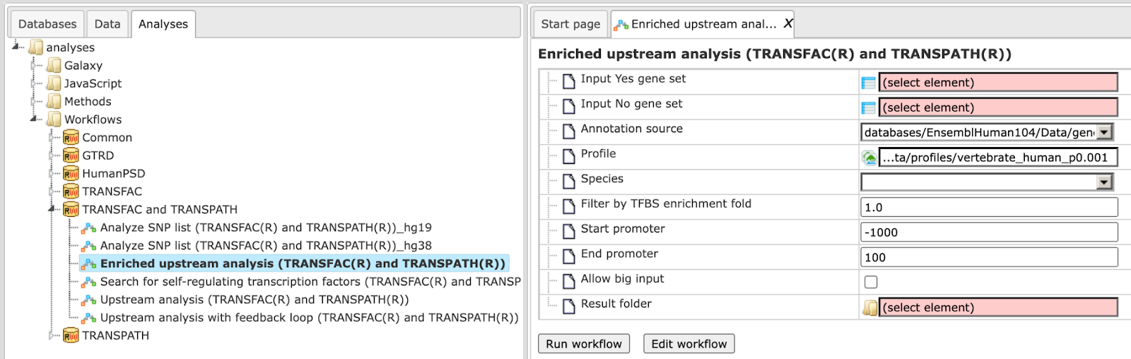
Step 1: Specify a gene set under study, e.g. a list of differentially regulated genes, as the Input Yes gene set. You can drag & drop it from your project within the Tree Area and drop in the pink box of the field Input gene set. Input gene set used for example
Step 2: Input a No gene set. This is the set of background genes or control set. The default. No set used for this workflow is data/Examples/Sample data/Data/Housekeeping genes (Human). If your Yes set is from mouse or rat, you may wish to adjust the No set accordingly.
Step 3: Define a TRANSFAC® profile. The default. profile is vertebrate_human_p0.001. Any other TRANSFAC® profile or user-specific profile can be chosen. With a mouse click on the field Profile, a pop-up window will open, where a profile can be selected.
Step 4: Specify the biological species of the input set in the field Species by selecting the required species from the drop-down menu.
Step 5: Filter by TFBS enrichment fold: In this field you can specify the enrichment fold (FE) to filter the motifs. By default., FE is 1.0, which means all motifs with FE>1.0 will be reported in the resulting table and the same motifs will serve to create a specific profile. If you want to use highly-enriched motifs, you can specify higher thresholds, e.g. 1.1, 1.2, or even 2.0 or 3.0 depending on your Yes and No sets. It is recommended that you run the workflow with default. parameters first, check the results, and then run again with the desired filter value.
Step 6: Define the length of the promoter regions to be analyzed. The default. promoter region is from-1000 to 100 relative to the TSS as annotated in the Ensembl database. You can adjust Start of promoter and End of promoter by typing in the corresponding fields.
Step 7: Checking Allow big input enables analysis of more than 500 promoters.
Step 8: Define where the folder with the results should be located in your project tree. You can do so by clicking on the pink box (select element) in the field Results folder, and a new window will open, where you can select the location of the results folder and define its name.
Step 9: Press the [Run workflow] button. Wait until the workflow is completed, and take a look at the results.
Visualization and interpretation of results
The Enriched Upstream Analysis result folder contains several files.
Enriched motifs
The list of motifs, which were identified during the first part of the workflow
and filtered with enrichment fold >1 can be found in the table
Enriched_motifs ( ). It contains those site models, here TRANSFAC® matrices, which are enriched in the Yes set in comparison with the No set as shown below:
The table Profile ( ) presents details for PWMs with adj. site FE >1. This profile is an intermediate result of the workflow and is used further for Site search on gene
set analysis.
) presents details for PWMs with adj. site FE >1. This profile is an intermediate result of the workflow and is used further for Site search on gene
set analysis.
Site search analysis output ( ) serves to visualize enriched motifs in the promoters. This folder contains four tracks (
 ). The output table Transcription factors Ensembl genes
is a list of transcription factors linked to the enriched motifs. For each transcription factor, the Ensembl gene ID is provided, as well gene description, HGNC gene symbol, species, and site model (TRANSFAC® PWM name).
This list of transcription factors is the input for the second part of the workflow, the master regulator search.
Master regulators
The primary result table Enriched Master regulators upstream 10 ( ) is a list of master regulatory molecules that were identified at a distance of up to 10 steps upstream of the input TFs. Each master regulatory molecule is
characterized by a Score, Z-score, FDR, and Ranks Sum.
) is a list of master regulatory molecules that were identified at a distance of up to 10 steps upstream of the input TFs. Each master regulatory molecule is
characterized by a Score, Z-score, FDR, and Ranks Sum.
The selection of the best master regulatory molecules based on Score, Z-score and Ranks sum is explained therein under “Interpretation of the results”.
The three Top 3 regulators diagrams ( ) visualize the networks for each of the three top master regulators. By default., the top regulators are identified upon sorting the Master regulators upstream 10 table
() by the column Ranks sum with the lowest rank on top.
) visualize the networks for each of the three top master regulators. By default., the top regulators are identified upon sorting the Master regulators upstream 10 table
() by the column Ranks sum with the lowest rank on top.
Note This workflow is available together with valid TRANSFAC® and TRANSPATH® licenses. Please feel free to ask for details (info@genexplain.com).
Upstream analysis (TRANSFAC(R) and TRANSPATH(R))
This workflow is a comprehensive promoter and pathway analysis. At the first step the promoters of differentially regulated genes are retrieved (-1000bp relative to TSS and +100bp relative to TSS) and analyzed for potential transcription factor (TF) binding sites. To identify enriched binding sites within the promoter sequences, positional weight matrices from the TRANSFAC(R) database are used while performing the method Site search on gene set. The site search result will be further converted into a table of transcription factors that potentially have regulated the DEGs. In the second step, the pathways are reconstructed with information about all relevant signaling cascades from the TRANSPATH® database and that are known to activate the previously hypothesized TFs. Molecules where these pathways converge are considered as potential master regulators of the biological process under study.
✨ Open the workflow in the user interface.✨
The following list gives an overview of all input parameters used in this workflow:
Parameter |
Description |
|---|---|
Input Yes gene set |
Input gene table |
Species |
Define the species of your data |
AnnotationSource |
Ensembl annotation source file |
Input No gene set |
Table with background genes |
Profile |
Collection of positional weight matrices from TRANSFAC(R) |
Start of promoter |
5 prime position relative to TSS (base pairs) |
End of promoter |
3 prime position relative to TSS (base pairs) |
Results folder |
Name and location of outputs |
A gene table (input example) can be submitted in the input field Input gene table (input example). You can drag and drop the input gene table from your data project within the tree area or you may click into the input field (select element) and a new window will be opened, where you can select your input table. The table can be in any format and will be converted into an Ensembl gene list.
You need to select the biological species of your data in the field Species by choosing the required one from the drop-down menu.
For gene annotation the most recent Ensembl database is used and set as default. for the workflow run. You can adapt the database version in the field AnnotationSource to your needs.
As a background set a gene table with 300 house-keeping genes will be automatically selected in the field Input No gene set and correspond to the species of your input gene table.
Please choose in the field Profile a collection of positional weight matrices from TRANSFAC(R) database for performing the search of enriched transcription factor binding sites (TFBSs) in your workflow run.
Specify the promoter region relative to the transcriptional start site (TSS) as they are annotated in Ensembl. The default. promoter region is -1000bp and +100bp relative to the TSS of a gene. You can edit the fields Start of promoter and End of promoter as required.
A result folder is generated and contains several tables. The identified enriched transcription factor binding sites (TFBSs) are present in a summary table (result example) with a matrix logo and the corresponding TF name. The potential transcription factors are given in a final table (result example) with annotated GeneSymbol IDs and a short description. From the second part of the workflow a list of master regulatory molecules (result example) is generated that were identified at a distance of up to 10 steps upstream of the input TFs. Each master regulatory molecule is characterized by a Score, Z-score, FDR, and Ranks sum.
The score value of each master regulatory molecule reflects how well this molecule is connected with other molecules in the database, and how many molecules from the input list are present in the network of this master molecule. The higher the Score value, the better is this molecule connected in the database, and the more “Hits” from the input list are present in the network of this molecule. By default., only the molecules with Score > 0.2 are shown in the output.
Because molecules with high Scores are well connected in the database, they are being suggested quite often by the tool as potential master regulators even with different input lists, and sometimes such molecules are also expected to be found a priori. It is possible to say that the molecules with the highest Score values are a kind of “trivial” and expected solutions. At the same time, and also because of their good connectivity, they are well studied and published. Therefore the molecules with high Score values might be biologically interesting as known “hubs” in a network.
Z-score
The Z-score value reflects how specific each master molecule is for the input list. The higher the Z-score value for a molecule, the more specific this molecule is for the input list, and the lesser is the probability to find such a molecule as master regulator in another analysis. Z-score and FDR are calculated based on 1000 random results, for which 1000 random input sets of the same size were generated by the algorithm.
Importantly, Score and Z-score reflect different characteristics of the suggested master regulators in the networks. Molecules with high Score values are well connected in the database, and therefore not very specific for the input list, and correspondingly they have quite moderate Z-score values.
Molecules with highest Z-scores are very specific for the input list, probably because of a few connections that are specific for the input list, but generally they are not so well connected within the database and therefore have quite low Score values.
Sorting by Z-score and considering top molecules might be helpful if you are interested in finding novel master regulators which are specific for your input list and generally are not well studied yet. By default., only the molecules with Z-score > 1.0 are shown in the output.
Ranks sum
This column helps to suggest molecules for which both values, Score and Z-score, are quite good. The column Ranks sum reflects a combination of sorting by Score and by Z-score in the following way.
Upon sorting by Score from biggest values to the lowest, a rank is assigned to the molecules; the molecule with the highest Score has rank 1, etc.
Upon independent sorting by Z-Score from biggest values to lowest, a rank is assigned to the molecules; the molecule with the highest Z-score has rank 1, etc.
Next, for each molecule, the ranks upon sorting by Score and upon sorting by Z-Score are summed up in the column Ranks Sum. The lower the Ranks sum, the more interesting the candidate molecule is, with good Score and good Z-score values.
By default., the table Master regulators upstream 10 are sorted by the Ranks sum column, to suggest molecules with a balance between their well-studied status and high connectivity (reflected by Score), and novelty and specificity for the input list (reflected by the Z-score).
The top three identified master regulators (with lowest Ranks sum) are visualized in reconstructed networks (result example).
If you are interested in finding reliable well-studied master regulators, e.g. to confirm already known ones, and would like a master regulator network to contain as many molecules from the input list as possible, you might be interested to sort by Score, and consider master molecules with the highest Score values.
If you are looking for novel master regulators that are very specific for your input list, even when they are not well studied yet, you might be interested to sort by Z-score, and consider master molecules with highest Z-score values.
If you are looking for a good balance between well-connected molecules and novel ones specific for your input list, you might be interested to stay with the default. sorting by Ranks sum, and consider master molecules with the lowest Ranks sum values.